Plotting of Spectral Fits and Models (model)

Spectral fits resulting from using SpectralFitter (see Spectral Fitting for details), can be plotted with the ModelFit plot class. This class will plot the fit results, and can show the resulting photon model in photon, energy, or \(\nu F_\nu\) space.

We will load an example spectral fit to demonstrate the plot capabilities:

>>> import os
>>> from gdt.core import data_path
>>> from gdt.core.spectra.fitting import SpectralFitterPgstat
>>> saved_fit = data_path.joinpath('specfit.npz')
>>> specfitter = SpectralFitterPgstat.load(saved_fit)
Fit loaded from 2023-03-01 20:41:59

>>> import matplotlib.pyplot as plt
>>> from gdt.core.plot.model import ModelFit
>>> modelplot = ModelFit(fitter=specfitter, interactive=True)
>>> plt.show()

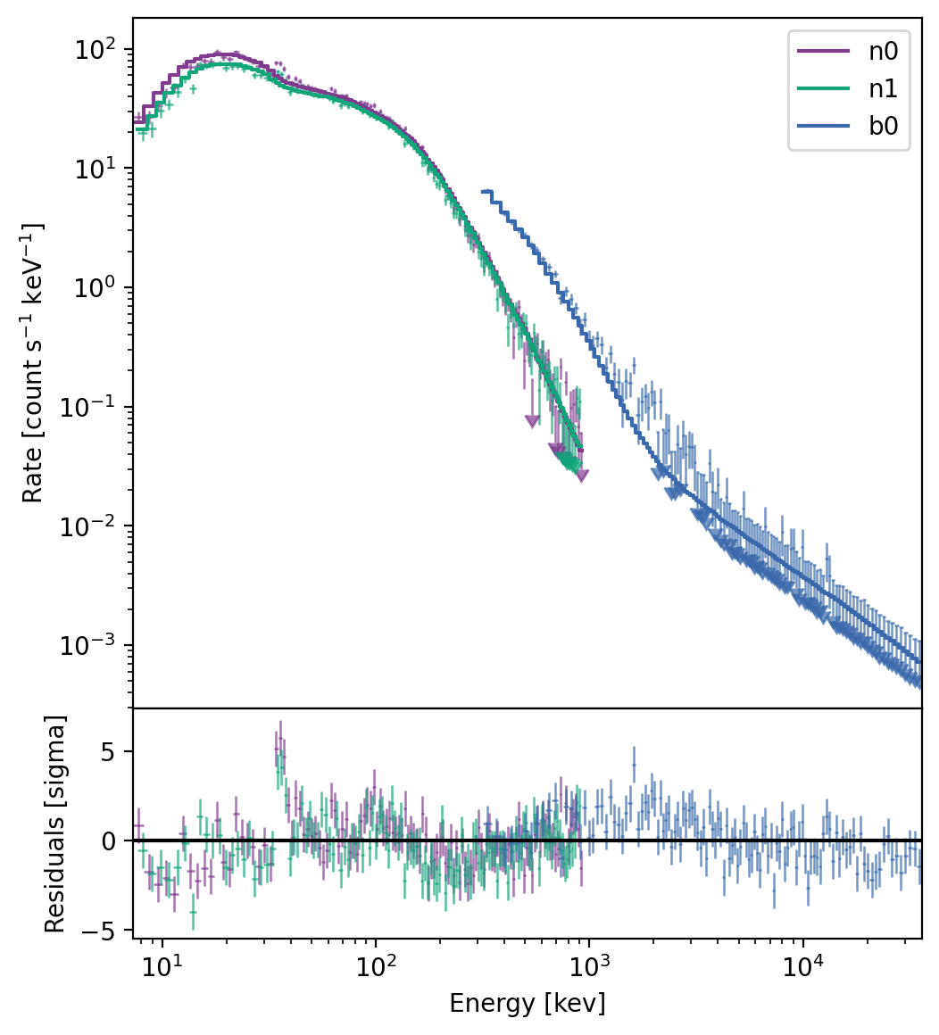
The default plot shows the different data sets, in this case data from three different Fermi GBM detectors. The histograms are the count rate spectral models, and the data points are the count rate data. By default, data points that are below the model variance are shown as 2 sigma upper limits. In the lower panel are the residuals in units of model standard deviation.

We can hide the residuals:

>>> modelplot.hide_residuals()

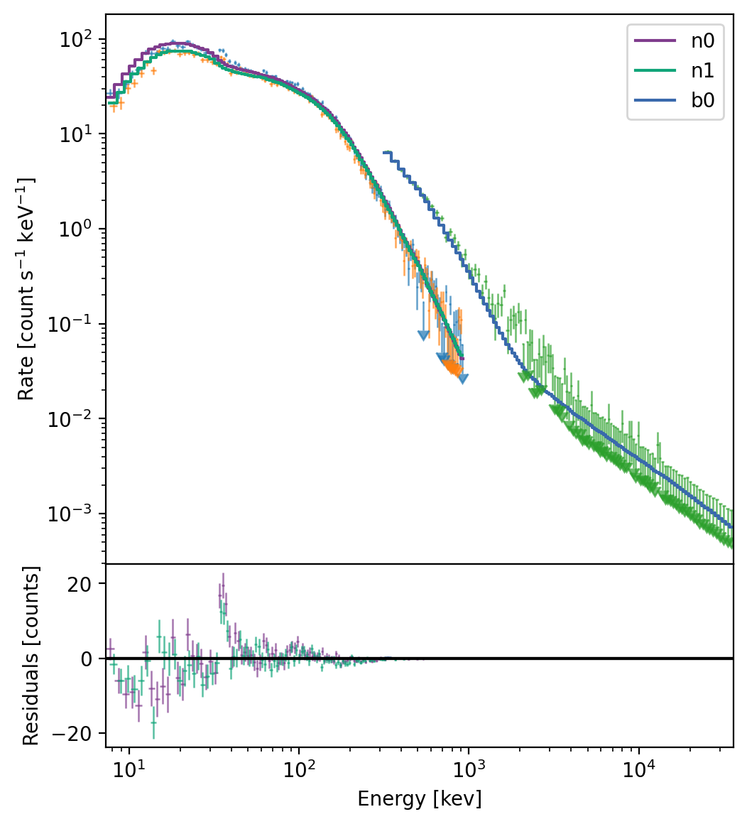
Or change the residuals to units of counts:

>>> modelplot.show_residuals(sigma=False)

There are three collections of plot objects on this plot: The count rate model which is stored as a PlotElementCollection of Histo objects, the count rate data, and the residuals, both of which are collections of ModelData objects.

>>> modelplot.count_models
<PlotElementCollection: 3 Histo objects>

>>> modelplot.count_data
<PlotElementCollection: 3 ModelData objects>

>>> modelplot.residuals
<PlotElementCollection: 3 ModelData objects>

Each of the plot elements can be accessed by the detector name they belong to:

>>>  modelplot.count_data.items
['n0', 'n1', 'b0']
>>> modelplot.count_data.get_item('n0')
<ModelData: color='#7F3C8D';
            alpha=0.7>
>>> modelplot.count_data.n1
<ModelData: color='#11A579';
            alpha=0.7>

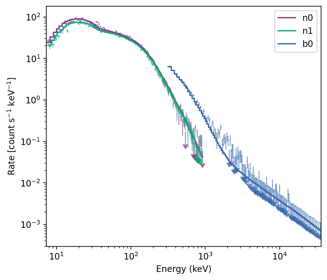
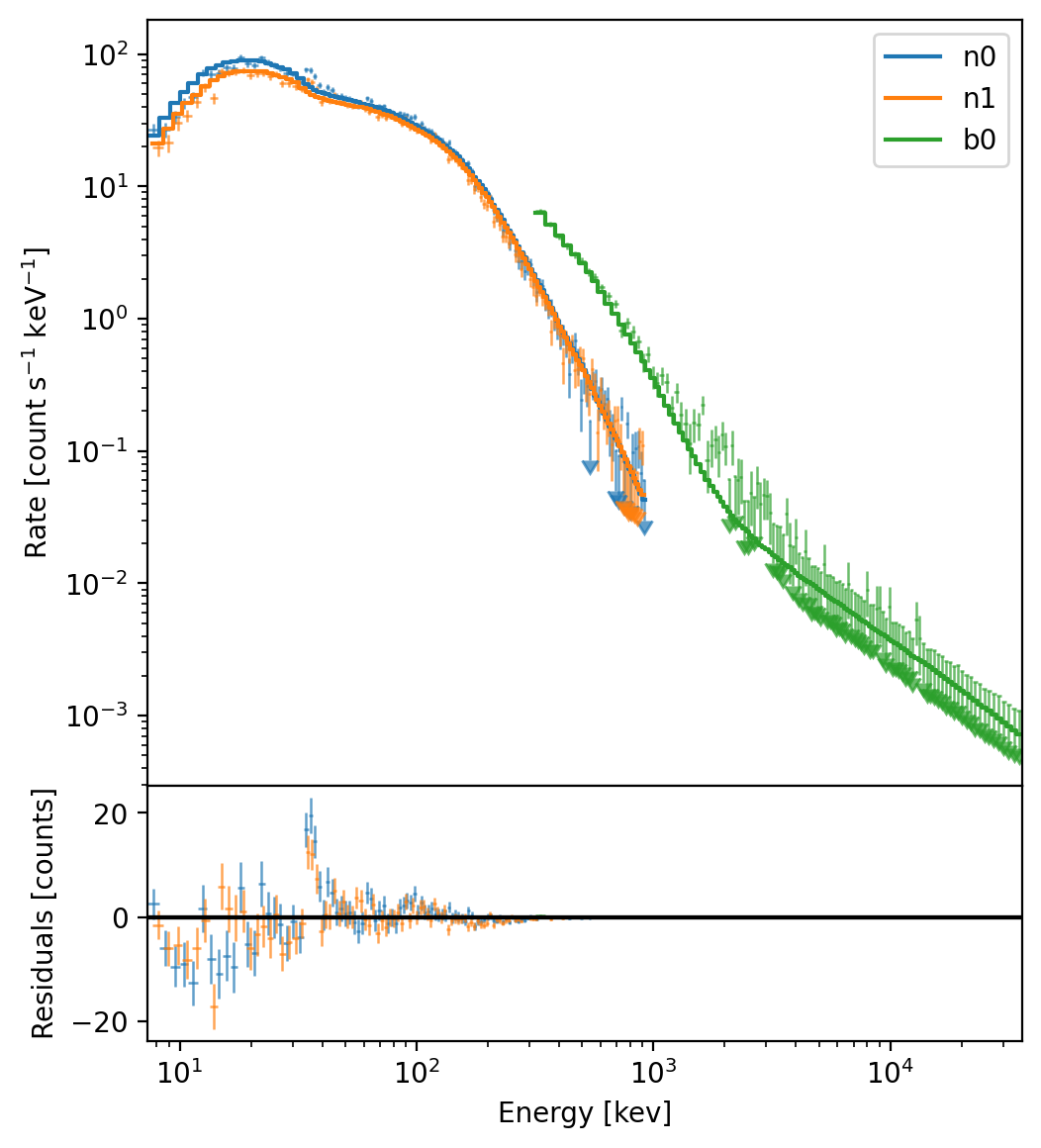
If we want to change the colors, we can do so by iterating over the items in the collection:

>>> colors = ['C0', 'C1', 'C2']
>>> for item, color in zip(modelplot.count_data, colors):
>>>     item.color = color

Of course, we need to update the colors for the count rate model and the residuals:

>>> for item, color in zip(modelplot.count_models, colors):
>>>     item.color = color

>>> for item, color in zip(modelplot.residuals, colors):
>>>     item.color = color

And unfortunately since Matplotlib doesn’t currently support updating the legend when the corresponding plot elements are changed, we need to update the legend as well:

>>> for item, color in zip(modelplot.ax.get_legend().legendHandles, colors):
>>>     item.set_color(color)

So far, we have only shown the count rate spectrum view, which is only one of four views that we can show on the plot. We can also plot the modeled photon spectrum:

>>> modelplot.photon_spectrum()

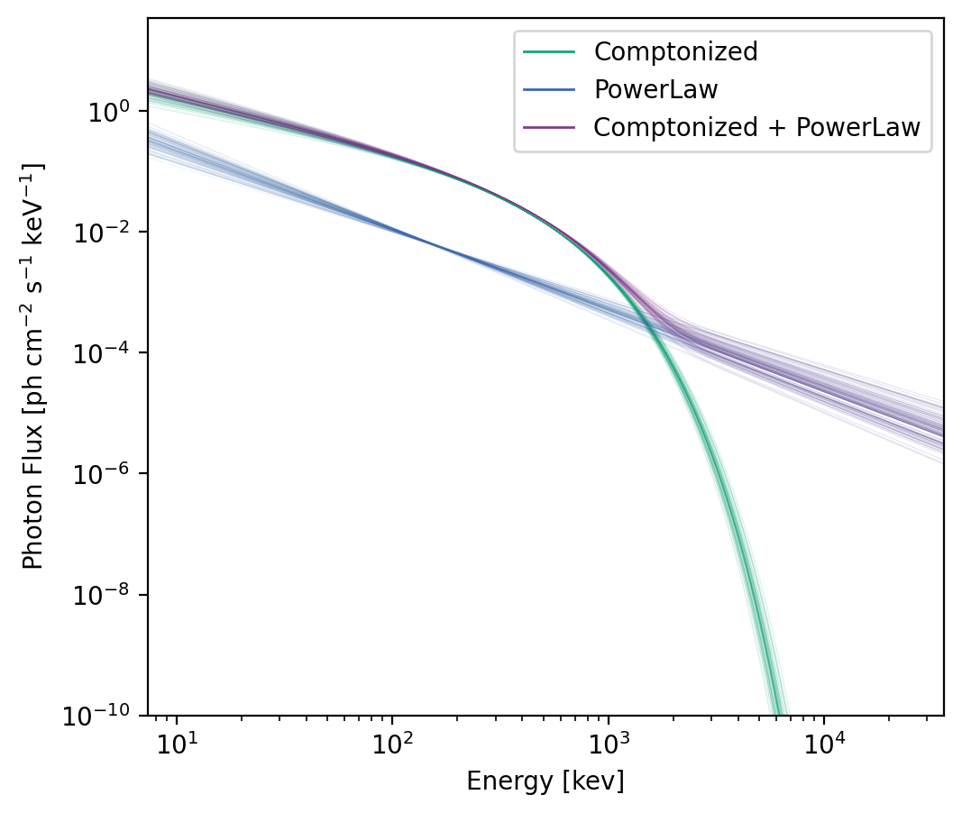
This view shows the differential photon flux as a function of energy. In our example, we have fit a multi-component model, and each component is shown, along with the combined model. Each component has several instances of the spectrum drawn from the covariance matrix of the fit. These are stored as a collection of ModelSamples objects:

>>> modelplot.spectrum_model
<PlotElementCollection: 3 ModelSamples objects>

We can change the colors in the same way we changed the colors in in the count spectrum view. And again, we will have to update the legend.

>>> colors = ['C0', 'C1', 'C2']
>>> for item, color in zip(modelplot.spectrum_model, colors):
>>>     item.color = color

>>> for item, color in zip(modelplot.ax.get_legend().legendHandles, colors):
>>>     item.set_color(color)

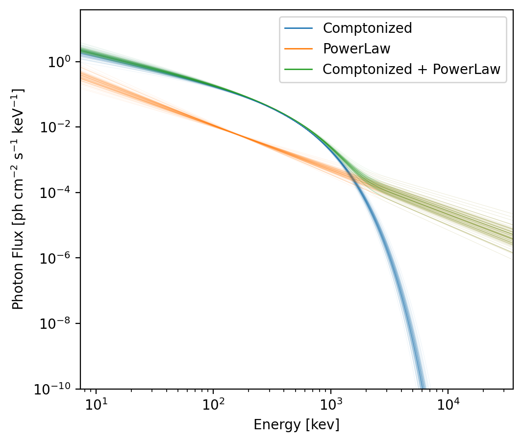
We can also plot the energy spectrum view. By default, multiple components are shown in each view, but we can turn those off. Also be default, 100 model samples are drawn to create the plot, but we can also changes this.

>>> modelplot.energy_spectrum(plot_components=False, num_samples=1000)

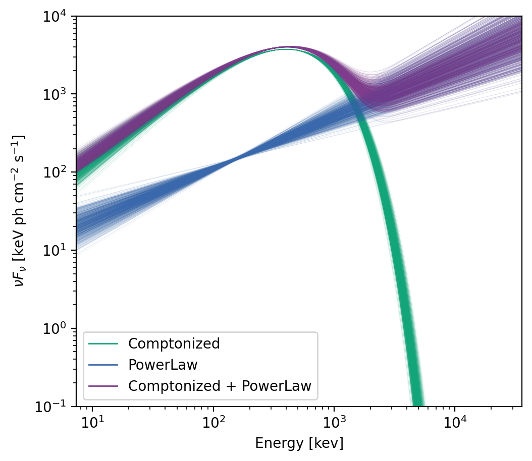
And finally, we can plot the \(\nu F_\nu\) spectrum:

>>> modelplot.nufnu_spectrum(num_samples=1000)
>>> modelplot.ylim = (0.1, 1e4)

Reference/API

gdt.core.plot.model Module

Classes

ModelFit([fitter, canvas, view, resid, ...])

Class for plotting spectral fits.

Class Inheritance Diagram