Plotting Sky Maps, Localizations, and Wide-field Effective Area (sky)

A plot of the observing scenario for an observatory condenses a lot of information into a single figure. The GDT provides a SkyPlot base class for the purpose of creating such a plot. There are three derived classes that plot the instrument observing conditions and data in different general frames:

• EquatorialPlot - Plotting the sky in the equatorial frame (GCRS)

• GalacticPlot - Plotting the sky in the Galactic frame

• SpacecraftPlot - Plotting the sky in the spacecraft inertial frame

In addition to these different frames, the sky plots can be made with the current compatible projections:

• Aitoff

• Hammer

• Lambert

• Mollweide

• Polar

Sky Maps

A sky map shows the observing scenario for the observatory instrument(s). This includes default plotting of Earth occultation, the location of the sun, the Galactic Plane, and the instrument pointings. In order to make such a plot, we will need a SpacecraftFrame object containing the spacecraft orientation information. As an example, we will read in a Fermi GBM position history file that contains this information (see Spacecraft Attitude, Position, and Coordinates for details about using the SpacecraftFrame class).

>>> from gdt.core import data_path
>>> from gdt.missions.fermi.gbm.poshist import GbmPosHistFile
>>> # get the spacecraft frame from the position history file
>>> filepath = data_path.joinpath('fermi-gbm').joinpath(('glg_poshist_all_170101_v01.fit')
>>> with GbmPosHistFile(filepath) as poshist:
>>>     frame = poshist.get_spacecraft_frame()

Now we will initialize the plot and add one of the frames to the plot. Let’s plot in equatorial coordinates.

>>> import matplotlib.pyplot as plt
>>> from gdt.core.plot.sky import EquatorialPlot
>>> eqplot = EquatorialPlot(interactive=True)
>>> # add the first frame from the Fermi position history file
>>> eqplot.add_frame(frame[0])
>>> plt.show()

There are several things on this plot to note. First, the blue blob is the region occulted by the Earth, and we can access the plot element, which is a SkyCircle:

>>> eqplot.earth
<SkyCircle: face_color=deepskyblue;
            face_alpha=0.25;
            edge_color=deepskyblue;
            edge_alpha=0.5;
            linestyle='solid';
            linewidth=1.0>

We can change the plot settings in the following way:

>>> eqplot.earth.color = 'purple'
>>> eqplot.earth.face_alpha = 0.5
>>> eqplot.earth.linewidth = 2

Next, the Fermi GBM detector pointings are shown in gray and are annotated with the detector numbers. Each detector is a DetectorPointing object, and they are all stored in a PlotElementCollection so that the properties can be set as a group. We can access each individual detector by using their name as the attribute of the collection.

>>> # the collection
>>> eqplot.detectors
<PlotElementCollection: 14 DetectorPointing objects>
>>> # the plot object for the 'n0' detector
>>> eqplot.detectors.n0
<DetectorPointing: 'n0';
               face_color=dimgray;
               face_alpha=0.25;
               edge_color=dimgray;
               edge_alpha=0.5;
               linestyle='solid';
               linewidth=1.0;
               fontsize=10;
               font_color=dimgray;
               font_alpha=0.8>

We can update the plot properties for all detectors at once by setting the corresponding attribute of the collection. Note that when we set an attribute of the collection, we must call it as a method:

>>> eqplot.detectors.face_color('green')
>>> eqplot.detectors.face_alpha(0.5)
>>> eqplot.detectors.edge_color('forestgreen')
>>> eqplot.detectors.font_color('purple')
>>> eqplot.detectors.fontsize(12)

We can update the properties of individual detectors, too:

>>> eqplot.detectors.n3.color = 'salmon'
>>> eqplot.detectors.n3.font_color = 'black'

The next item on the plot is the sun, which is now unfortunately hidden behind our darker detector circles. We can fix that by accessing the Sun plot element:

>>> eqplot.sun
<Sun: alpha=1.0;
  size=150.0>

>>> eqplot.sun.zorder = 10
>>> eqplot.sun.size = 300

Finally, the stylized galactic plane plot element is a GalacticPlane object:

>>> eqplot.galactic_plane
<GalacticPlane: outer_color=dimgray;
                inner_color=black;
                line_alpha=0.5;
                center_alpha=0.75;

And we can similarly update the plot properties:

>>> eqplot.galactic_plane.outer_color = 'red'
>>> eqplot.galactic_plane.inner_color = 'darkred'
>>> eqplot.galactic_plane.line_alpha = 0.7
>>> eqplot.galactic_plane.zorder = 0

We can also make the plot in the Galactic frame:

>>> from gdt.core.plot.sky import GalacticPlot
>>> galplot = GalacticPlot(interactive=True)
>>> galplot.add_frame(frame[0])

And also in the spacecraft frame, where the longitudinal coordinates are the spacecraft azimuth and the latitudinal coordinates are relative to spacecraft zenith (i.e. zenith=0 is often the “top” or boresight of the observatory).

>>> from gdt.core.plot.sky import SpacecraftPlot
>>> scplot = SpacecraftPlot(interactive=True)
>>> scplot.add_frame(frame[0])

Localizations

We can also visualize localizations on these sky maps by adding a HealPixLocalization object to our plot. In our example, we will read in a Fermi GBM localization (see The HealPix Module for more information about using HealPixLocalization objects).

>>> from gdt.missions.fermi.gbm.localization import GbmHealPix
>>> filepath = data_path.joinpath('fermi-gbm/glg_healpix_all_bn190915240_v00.fit')
>>> loc = GbmHealPix.open(filepath)

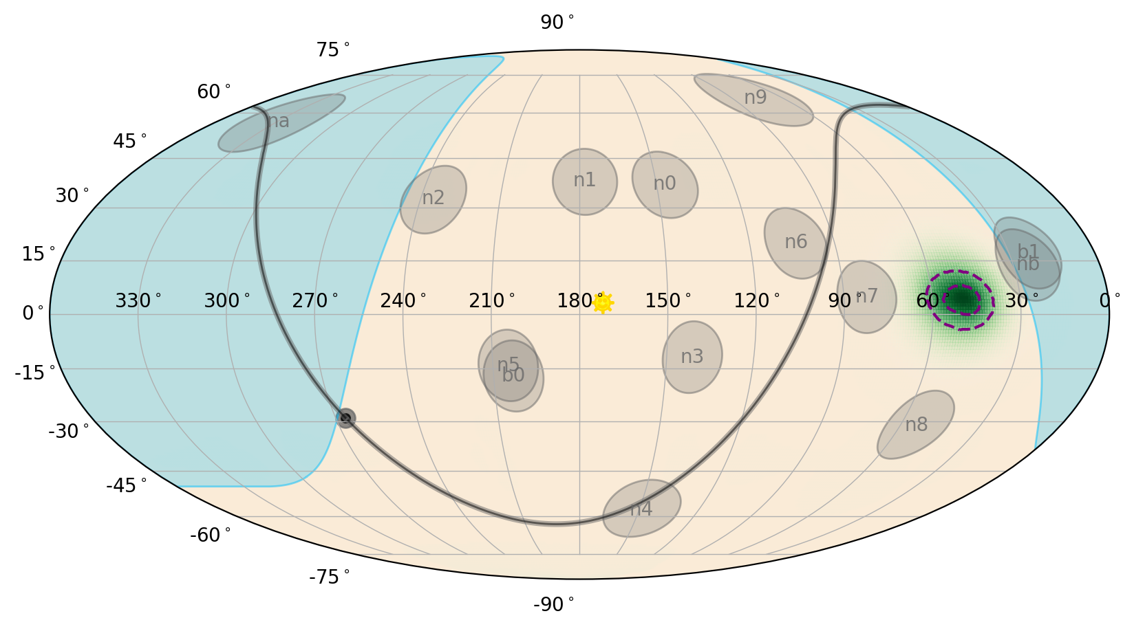
Now we simply create our plot and add the localization”

>>> eqplot = EquatorialPlot(interactive=True)
>>> eqplot.add_localization(loc, gradient=True, clevels=[0.5, 0.9])

In this example, we have set the localization posterior to be plotted as a gradient and have marked the 50% and 90% confidence regions. The posterior, which is a SkyHeatmap object, can be accessed and updated:

>>> eqplot.loc_posterior
<SkyHeatmap: color='RdPu';
             norm=PowerNorm>

>>> from matplotlib.colors import PowerNorm
>>> # effectively decrease the sharpness of the color gradient norm
>>> eqplot.loc_posterior.norm = PowerNorm(gamma=0.2)
>>> eqplot.loc_posterior.color.name = 'Greens'

The localization contours are stored in a PlotElementCollection as SkyLine objects and can be updated in a similar way to how we updated the detectors:

>>> eqplot.loc_contours.color('purple')
>>> eqplot.loc_contours.alpha(1.0)
>>> eqplot.loc_contours.linewidth(1.5)
>>> eqplot.loc_contours.linestyle('--')

Instead of plotting the gradient of the localization posterior, we can plot stacked filled contours instead:

>>> eqplot = EquatorialPlot(interactive=True)
>>> eqplot.add_localization(loc, gradient=False, clevels=[0.5, 0.9, 0.99])

As with the non-filled contours, these are stored in a PlotElementCollection, but are SkyPolygon objects:

>>> eqplot.loc_contours
<PlotElementCollection: 3 SkyPolygon objects>
>>> eqplot.loc_contours.items
['0.5_0', '0.9_0', '0.99_0']

Note

The item names here are <clevel>_<segment number> where segment number may be > 0 when the contour is split across the sky meridian. Because these names have a period in them, they cannot be accessed as an attribute, so use the standard get_item() method.

>>> eqplot.loc_contours.get_item('0.5_0')
<SkyPolygon: face_color=purple;
             face_alpha=0.3;
             edge_color=purple;
             edge_alpha=None;
             linestyle='-';
             linewidth=1.5>

We can update the contour properties in the normal way:

>>> eqplot.loc_contours.face_color('green')
>>> eqplot.loc_contours.edge_color('green')
>>> eqplot.loc_contours.linestyle('--')

Finally, we can demonstrate plotting the localization in a different projection altogether. Let’s plot the localization in the spacecraft frame and in a polar projection:

>>> # reduce the polar tick resolution
>>> scplot = SpacecraftPlot(interactive=True, projection='polar', yticks_res=30)
>>> scplot.add_localization(loc, gradient=False, clevels=[0.5, 0.9, 0.99])

Effective Area

All-sky or wide-field angular responses can be plotted on a sky map as well. To do so, we utilize the HealPixEffectiveArea class, which contains the effective area on the sky (see The HealPix Module for more information about using HealPixEffectiveArea objects).

For our example, we will create a cosine-like idealized response:

>>> from gdt.core.healpix import HealPixEffectiveArea
>>> # peak effective area of 100 cm^2 at az=60, zen=90
>>> effarea = HealPixEffectiveArea.from_cosine(60.0, 90.0, 100.0, coeff=2.0)

Next we can add it a sky plot. Let’s plot in spacecraft coordinates:

>>> scplot = SpacecraftPlot(interactive=True)
>>> scplot.add_effective_area(effarea)

Similar to the localization posterior gradient, the effective area is a SkyHeatmap object and the same properties can be set:

>>> scplot.effective_area
<SkyHeatmap: color='RdPu';
             norm=PowerNorm>

To plot in other coordinate frames, we need to provide a SpacecraftFrame so that the effective area can be rotated into that frame. We can also plot all of the normal things on the sky as well:

>>> galplot = GalacticPlot(interactive=True)
>>> galplot.add_effective_area(effarea, frame=frame[0], earth=True, sun=True,
>>>                            galactic_plane=True)

Reference/API

gdt.core.plot.sky Module

Classes

SkyPlot([projection, flipped, xticks_res, ...])	Base class for an all-sky plot.
EquatorialPlot([projection, flipped, ...])	Plotting the sky in Equatorial (GCRS) coordinates.
GalacticPlot([projection, flipped, ...])	Plotting the sky in Galactic coordinates.
SpacecraftPlot([zenith])	Class for plotting the sky in Spacecraft coordinates.

Class Inheritance Diagram