Data Primitives (gdt.core.data_primitives)

Introduction

The data primitives are the data classes that define the datatypes within the GDT at the most basic level.

Range and Intervals

A value covering a defined interval, such as time interval or energy range, can be represented by a Range. Two specific types of Ranges are provided: EnergyRange and TimeRange. A series of Ranges are represented by an Intervals object. Similar to the energy- and time-specific Range classes, there are energy- and time-specific classes: Ebounds and Gti, respectively.

Examples

To create a Range object:

>>> from gdt.core.data_primitives import EnergyRange, TimeRange
>>> erange = EnergyRange(50.0, 300.0)
>>> erange
<EnergyRange: (50.0, 300.0)>
>>> trange = TimeRange(-10.0, 10.0)
>>> trange
<TimeRange: (-10.0, 10.0)>

You can check to see if the Range contains a particular value:

>>> erange.contains(100.0)
True
>>> trange.contains(10.0)
True
>>> trange.contains(10.0, inclusive=False)
False

The intersection or union of two Ranges can also be computed to return a new Range:

>>> erange2 = EnergyRange(250.0, 500.0)
>>> EnergyRange.intersection(erange, erange2)
<EnergyRange: (250.0, 300.0)>
>>> trange2 = TimeRange(30.0, 100.0)
>>> TimeRange.union(trange, trange2)
<TimeRange: (-10.0, 100.0)>

Often one is working with a series of ranges, or intervals. As mentioned previously, the Gti class, (Good Time Intervals) is used for a set of time intervals, and the Ebounds class is used for a set of energy intervals. There are a few ways to create an Intervals object:

>>> from gdt.core.data_primitives import Ebounds, Gti
>>> ebounds1 = Ebounds(erange)
>>> ebounds1
<Ebounds: 1 intervals; range (50.0, 300.0)>
>>> gti1 = Gti.from_bounds((-10.0, 0.0, 10.0), (-5.0, 5.0, 15.0))
>>> gti1
<Gti: 3 intervals; range (-10.0, 15.0)>
>>> gti2 = Gti.from_list([(20.0, 25.0), (50.0, 55.0)])
>>> gti2
<Gti: 2 intervals; range (20.0, 55.0)>

In the first case, an Intervals object is initialized with a Range object. The second scenario creates an Intervals object from a list of lower and upper bounds, while the final scenario creates the object from a list of lower/upper tuples. Once initialized, the ranges can be retrieved as a list or individually:

>>> gti1.intervals
[<TimeRange: (-10.0, -5.0)>,
 <TimeRange: (0.0, 5.0)>,
 <TimeRange: (10.0, 15.0)>]
>>> gti1[1]
<TimeRange: (0.0, 5.0)>

Similar to the Range classes, you can check if a value is contained in the intervals:

>>> gti1.contains(5.0)
True
>>> gti1.contains(6.0)
False

A new Range can be inserted into the intervals:

>>> gti1.insert(TimeRange(7.0, 8.0))
>>> gti1.intervals
[<TimeRange: (-10.0, -5.0)>,
 <TimeRange: (0.0, 5.0)>,
 <TimeRange: (7.0, 8.0)>,
 <TimeRange: (10.0, 15.0)>]

Or two Intervals can be merged into one:

>>> gti_merged = Gti.merge(gti1, gti2)
>>> gti_merged
<Gti: 6 intervals; range (-10.0, 55.0)>

Finally, the we can perform the intersection of two intervals:

>>> gti3 = Gti(TimeRange(4.0, 12.0))
>>> gti_intersect = Gti.intersection(gti_merged, gti3)
>>> gti_intersect.intervals
[<TimeRange: (4.0, 5.0)>, <TimeRange: (10.0, 12.0)>]

1D Binned Data

A set of intervals with a corresponding value for each interval, such as the number of items in a series of bins, can be represented by a Bins object. This is essentially a type of histogram with a variety of useful properties and methods. A useful, specialized histogram for containing gamma-ray data is defined by the ExposureBins class. This class modifies Bins by incorporating an exposure for each bin. Furthermore, distinct ChannelBins, EnergyBins, and TimeBins classes are used to contain spectral and temporal data.

Examples

To create a TimeBins or EnergyBins, you need to initialize with an array of counts in each bin, the lower bin edges, upper bin edges, and the exposure for each bin:

>>> from gdt.core.data_primitives import TimeBins, EnergyBins
>>> counts = [1, 2, 3, 2, 1, 0]
>>> low_edges = [0.1, 0.2, 0.3, 0.4, 0.5, 0.6]
>>> high_edges = [0.2, 0.3, 0.35, 0.5, 0.6, 0.7]
>>> exposure = [0.08, 0.08, 0.04, 0.08, 0.08, 0.08]
>>> time_bins = TimeBins(counts, low_edges, high_edges, exposure)
>>> time_bins
<TimeBins: 6 bins;
 range (0.1, 0.7);
 2 contiguous segments>

Notice in this example that there is a gap between the bins resulting in two distinct, contiguous segments. Those segments can be directly accessed:

>>> time_bins.contiguous_bins()
[<TimeBins: 3 bins;
  range (0.1, 0.35);
  1 contiguous segments>,
 <TimeBins: 3 bins;
  range (0.4, 0.7);
  1 contiguous segments>]

A variety of properties are available, such as the rate, uncertainty, and bin centroids:

>>> time_bins.rates
array([12.5, 25. , 75. , 25. , 12.5,  0. ])
>>> time_bins.rate_uncertainty
array([12.5, 17.67766953, 43.30127019, 17.67766953, 12.5, 0.])
>>> time_bins.centroids
array([0.15 , 0.25 , 0.325, 0.45 , 0.55 , 0.65 ])

Several operations can be performed, including taking slices of the TimeBins and merging multiple TimeBins:

>>> slice1 = time_bins.slice(0.1, 0.25)
>>> slice1
<TimeBins: 2 bins;
 range (0.1, 0.3);
 1 contiguous segments>

>>> slice2 = time_bins.slice(0.5, 0.8)
>>> slice2
<TimeBins: 2 bins;
 range (0.5, 0.7);
 1 contiguous segments>

>>> merged = TimeBins.merge([slice1, slice2])
>>> merged
<TimeBins: 4 bins;
 range (0.1, 0.7);
 2 contiguous segments>

TimeBins can also be rebinned using s binning function. For example, we can rebin our time_bins by a factor of 3:

>>> from gdt.core.binning.binned import combine_by_factor
>>> rebinned = time_bins.rebin(combine_by_factor, 3)
>>> rebinned
<TimeBins: 2 bins;
 range (0.1, 0.7);
 2 contiguous segments>
>>> rebinned.counts
array([6, 3])

Multiple TimeBins can be summed as long as they have the same bin edges:

>>> summed = TimeBins.sum([time_bins, time_bins])
>>> time_bins.counts
array([1, 2, 3, 2, 1, 0])
>>> summed.counts
array([2, 4, 6, 4, 2, 0])

An EnergyBins object can be created in the same way as a TimeBins object. There are a few small differences to consider. The bin centroids attribute returns the geometric bin centroids instead of the arithmetic centroids. There are also two additional attributes for the differential rate per keV and the associated uncertainty:

>>> counts = [1, 2, 3, 2, 1, 0]
>>> low_edges = [10.0, 20.0, 40.0, 80.0, 160.0, 320.0]
>>> high_edges = [20.0, 40.0, 80.0, 160.0, 320.0, 640.0]
>>> exposure = 10.0
>>> energy_bins = EnergyBins(counts, low_edges, high_edges, exposure)
>>> energy_bins
<EnergyBins: 6 bins;
 range (10.0, 640.0);
 1 contiguous segments>
>>> energy_bins.centroids
array([ 14.14213562,  28.28427125,  56.56854249, 113.13708499,
       226.27416998, 452.54833996])
>>> energy_bins.rates_per_kev
array([0.01    , 0.01    , 0.0075  , 0.0025  , 0.000625, 0.      ])

In the case were we don’t have an energy calibration and instead only have counts in a series of energy channels, we use a ChannelBins object.

>>> from gdt.core.data_primitives import ChannelBins
>>> counts = [1, 2, 3, 2, 1, 0]
>>> chan_nums = [0, 1, 2, 3, 4, 5]
>>> exposure = 10.0
>>> channel_bins = ChannelBins.create(counts, chan_nums, exposure)
>>> channel_bins
<ChannelBins: 6 bins;
 range (0, 5);
 1 contiguous segments>

The concept of bin edges is replaced by a channel number, therefore, we can still perform slicing and rebinning in the same way we do with EnergyBins:

>>> # slice and return channels 1-3
>>> channel_bins.slice(1, 3)
<ChannelBins: 3 bins;
 range (1, 3);
 1 contiguous segments>

>>> # rebin by factor of 3
>>> rebinned_channel_bins = channel_bins.rebin(combine_by_factor, 3)
>>> rebinned_channel_bins
<ChannelBins: 2 bins;
 range (0, 3);
 1 contiguous segments>

One behavior you should take note in rebinning ChannelBins is that the channel numbers are not renumbered:

>>> rebinned_channel_bins.chan_nums
array([0, 3])
>>> rebinned_channel_bins.size
2

2D Binned Data

We extend the philosophy of 1D time or energy data to 2D time and energy data in the TimeChannelBins and TimeEnergyBins classes. These data type are essentially 2D histograms, where one axis is time, and the other is energy, and the corresponding attributes and methods are available for the respective axes. Additionally, this class has the ability to integrate along either axis to produce a TimeBins or ChannelBins/EnergyBins.

Examples

To create a TimeEnergyBins object, you need a 2D array of counts, the time bin edges, exposure in each bin, and energy bin edges:

>>> from gdt.core.data_primitives import TimeEnergyBins
>>> counts = [[1, 4, 1], [2, 3, 0], [3, 2, 1], [4, 1, 2]]
>>> tstart = [0.1, 0.2, 0.3, 0.4]
>>> tstop = [0.2, 0.3, 0.4, 0.5]
>>> exposure = [0.8, 0.8, 0.8, 0.8]
>>> emin = [10.0, 20.0, 40.0]
>>> emax = [20.0, 40.0, 80.0]
>>> te_bins = TimeEnergyBins(counts, tstart, tstop, exposure, emin, emax)
>>> te_bins
<TimeEnergyBins: 4 time bins;
 time range (0.1, 0.5);
 1 time segments;
 3 energy bins;
 energy range (10.0, 80.0);
 1 energy segments>

Attributes similar to those for the 1D counterparts of this data type are available. For example:

>>> te_bins.energy_centroids
array([14.14213562, 28.28427125, 56.56854249])
>>> te_bins.time_centroids
array([0.15, 0.25, 0.35, 0.45])

Methods to slice, merge, and rebin along either axis are also available. You can integrate along either axis, as well:

>>> time_bins = te_bins.integrate_energy()
>>> time_bins
<TimeBins: 4 bins;
 range (0.1, 0.5);
 1 contiguous segments>

>>> energy_bins = te_bins.integrate_time()
>>> energy_bins
<EnergyBins: 3 bins;
 range (10.0, 80.0);
 1 contiguous segments>

TimeChannelBins are initialized in the same way, but instead of energy bin edges, the object is initialized with channel numbers:

>>> from gdt.core.data_primitives import TimeChannelBins
>>> counts = [[1, 4, 1], [2, 3, 0], [3, 2, 1], [4, 1, 2]]
>>> tstart = [0.1, 0.2, 0.3, 0.4]
>>> tstop = [0.2, 0.3, 0.4, 0.5]
>>> exposure = [0.8, 0.8, 0.8, 0.8]
>>> chan_nums = [0, 1, 2]
>>> tc_bins = TimeChannelBins(counts, tstart, tstop, exposure, chan_nums)
>>> tc_bins
<TimeChannelBins: 4 time bins;
 time range (0.1, 0.5);
 1 time segments;
 3 channels;
 channel range (0, 2);
 1 channel segments>

Most attributes and methods are the same between TimeChannelBins and TimeEnergyBins, with the exception of some of the attributes associated with the energy axis. We can integrate over either axis (note that integrating over time will return a ChannelBins object).

>>> # create lightcurve
>>> tc_bins.integrate_channels(chan_min=1, chan_max=3)
<TimeBins: 4 bins;
 range (0.1, 0.5);
 1 contiguous segments>

>>> # create energy channel spectrum
>>> tc_bins.integrate_time()
<ChannelBins: 3 bins;
 range (0, 2);
 1 contiguous segments>

We can rebin the energy channels:

>>> tc_bins.rebin_channels(combine_by_factor, 2)
<TimeChannelBins: 4 time bins;
time range (0.1, 0.5);
1 time segments;
1 channels;
channel range (0, 0);
1 channel segments>

And we can slice by energy channel:

>>> tc_bins.slice_channels(1, 3)
<TimeChannelBins: 4 time bins;
 time range (0.1, 0.5);
 1 time segments;
 2 channels;
 channel range (1, 2);
 1 channel segments>

TimeChannelBins has the additional function that allows us to apply an energy calibration via an Ebounds object and return a TimeEnergyBins object:

>>> emin = [10.0, 20.0, 40.0]
>>> emax = [20.0, 40.0, 80.0]
>>> ebounds = Ebounds.from_bounds(emin, emax)
>>> te_bins = tc_bins.apply_ebounds(ebounds)
>>> te_bins
<TimeEnergyBins: 4 time bins;
 time range (0.1, 0.5);
 1 time segments;
 3 energy bins;
 energy range (10.0, 80.0);
 1 energy segments>

Event Data

Instead of data binned in time, individual counts or photons may be recorded. These individual events have at least a time and energy attribute. Data like this are represented by an EventList. Typically these data are consider pseudo-unbinned, since they are truly unbinned in time, but are typically associated with binned energy channels. Similar to the other data types, the EventList has a variety of attributes and methods, including a bin() method that bins the EventList in time to produce a TimeEnergyBins object.

Examples

To create an EventList, an array of event timestamps is required, as well as a corresponding energy channel number for each event. Optionally, an Ebounds representing the channel-number-to-energy mapping can be provided:

>>> import numpy as np
>>> from gdt.core.data_primitives import EventList, Ebounds
>>> times = np.random.exponential(1.0, size=100).cumsum()
>>> channels = np.random.randint(0, 4, size=100)
>>> ebounds = Ebounds.from_bounds([10.0, 20.0, 40.0, 80.0], [20.0, 40.0, 80.0, 160.0])
>>> event_list = EventList(times, channels, ebounds=ebounds)
>>> event_list
<EventList: 100 events;
 time range (1.187301739254875, 100.5554859990595);
 channel range (0, 3)>

In this example, we generated 100 random times from a Poisson rate of 1 count/sec, and generated random energy channels from a 4-channel spectrum.

We can calculate the exposure of the EventList for the entire list or for a time range. Also, if there as in event deadtime, we can account for that:

>>> event_list.get_exposure(event_deadtime=2.6e-6)  # deadtime of 2.6 microsec
99.36797885980462
>>> event_list.get_exposure(time_ranges=[20.0, 30.0], event_deadtime=2.6e-6)
9.9999818

The EventList can be sliced in time, by channel, or energy range (if there is an associated Ebounds):

>>> time_sliced = event_list.time_slice(20.0, 30.0)
>>> time_sliced
<EventList: 10 events;
 time range (20.937084880954618, 29.304071460921584);
 channel range (0, 3)>

>>> channel_sliced = event_list.channel_slice(0, 1)
>>> channel_sliced
<EventList: 47 events;
 time range (2.018746928409505, 100.5554859990595);
 channel range (0, 1)>

>>> energy_sliced = event_list.energy_slice(50.0, 150.0)
>>> energy_sliced
<EventList: 53 events;
 time range (1.187301739254875, 96.20611692399264);
 channel range (2, 3)>

Multiple EventLists can be merged into a single list:

>>> merged = EventList.merge([channel_sliced, energy_sliced], force_unique=True)
>>> merged
<EventList: 100 events;
 time range (1.187301739254875, 100.5554859990595);
 channel range (0, 3)>

Given an algorithm to bin the event data, we can convert the EventList to a TimeEnergyBins:

>>> from gdt.core.binning.unbinned import bin_by_time
# bin to 10 s resolution, with an event deadtime of 2.6 microsec
>>> te_bins = event_list.bin(bin_by_time, 10.0, event_deadtime=2.6e-6)
>>> te_bins
<TimeEnergyBins: 10 time bins;
 time range (1.187301739254875, 101.18730173925488);
 1 time segments;
 4 energy bins;
 energy range (10.0, 160.0);
 1 energy segments>

Even without converting to a TimeEnergyBins, we can readily extract the count spectrum from the EventList:

>>> count_spec = event_list.count_spectrum(event_deadtime=2.6e-6)
>>> count_spec
<EnergyBins: 4 bins;
 range (10.0, 160.0);
 1 contiguous segments>

Note that if the energy calibration (ebounds) is not set for EventList, the bin() method will return a TimeChannelBins object and the count_spectrum() methods returns a ChannelBins object.

Response Matrix

A response matrix is a matrix that represents a detector energy response. Typically, a detector’s response will modify the incident spectrum so that the recorded spectrum is a convolution of the true incident spectrum with the detector response. Many factors may go into the calculation of the response matrix, such as energy dispersion, photon scattering, and absorption. Additionally, the magnitude of the response matrix is the effective area of the detector as a function of energy, accounting for factors such as the quantum efficiency of the detector. Often the response matrix contains significant off-diagonal contributions, which prevents matrix inversion, therefore estimates of the incident spectrum must be made indirectly via forward-folding techniques.

Examples

To create a ResponseMatrix object, we need to provide a 2D array of effective areas that correspond to the number of incident photon bins and the number of output energy channels. We also need to provide the incident photon bin edges and the output energy channel edges. In our simple example, we will create a simple diagonal response where the input and output edges are the same:

>>> import numpy as np
>>> from gdt.core.data_primitives import ResponseMatrix
>>> matrix = np.diag([0.1, 0.2, 0.3, 0.2, 0.1, 0.1])
>>> emin = [10., 20., 40., 80., 160., 320.]
>>> emax = [20., 40., 80., 160., 320., 640.]
>>> chanlo = emin
>>> chanhi = emax
>>> rsp = ResponseMatrix(matrix, emin, emax, chanlo, chanhi)
>>> rsp
<ResponseMatrix: 6 energy bins; 6 channels>

Similar to the other data primitives, there are several attributes provided. For example:

>>> rsp.channel_bin_centroids
array([ 14.14213562,  28.28427125,  56.56854249, 113.13708499,
       226.27416998, 452.54833996])
>>> rsp.photon_bin_widths
array([ 10.,  20.,  40.,  80., 160., 320.])

The effective area can be estimated at any arbitrary energy within the bounds of the response:

>>> rsp.effective_area(50.0)
0.2710806010829534
>>> rsp.effective_area(135.)
0.12418578120734841

Most importantly, any photon model can be folded through the response to produce the detector-convolved count spectrum. While you can certainly write a simple photon model function to fold through the response, there are built-in models in the spectral functions module. In our example, we will fold a power law through our response:

>>> from gdt.core.spectra.functions import PowerLaw
>>> pl = PowerLaw()
>>> # amplitude = 0.1; index = -2.2
>>> count_spectrum = rsp.fold_spectrum(pl.fit_eval, (0.1, -2.2))
>>> count_spectrum
array([7.39378818, 6.43666647, 4.20258271, 1.21952025, 0.26541351,
   0.11552794])

Thus, we have produced the count spectrum in counts/s.

The response can also be rebinned along the channel axis, if desired. This may be useful in cases where the corresponding spectral data is rebinned, although keep in mind that rebinning causes loss of information. To rebin the response, we specify either the factor at which to combine bins or a list of bin edge indices defining the bin edges that will remain after rebinning:

>>> rebinned_factor = rsp.rebin(factor=2) # rebin by factor of 2
>>> rebinned_factor
<ResponseMatrix: 6 energy bins; 3 channels>

>>> rebinned_edges = rsp.rebin(edge_indices=[0, 1, 5])
>>> rebinned_edges
<ResponseMatrix: 6 energy bins; 2 channels>

Finally, the input energy axis of the response can be resampled to increase or decrease the photon energy resolution or redefine the input photon bin edges. Keep in mind that this may introduce a systematic error via interpolation of the response, so you should always check to make sure the response behaves as expected after resampling. To resample, you can either specify the number of photon bins you want, in which case the bin edges are spaced logarithmically, or you can specify the edges of the bins. The photon bins can only be resampled within the energy bounds of the original response:

>>> resampled_num = rsp.resample(num_photon_bins=12)
>>> resampled_num
<ResponseMatrix: 12 energy bins; 6 channels>

>>> resampled_edges = rsp.resample(photon_bin_edges=(10., 30., 90., 640.))
>>> resampled_edges
<ResponseMatrix: 3 energy bins; 6 channels>

Parameter

A parameter in the context of the GDT is a variable that has an associated uncertainty regarding its value, and usually results from a fit to data. The Parameter class is a simple container for a value and the associated uncertainty and provides a few functions and different representations of the parameter.

Examples

To create a Parameter object, we need to provide at least a value and the 1-sigma equivalent uncertainty. We can also provide other useful information, such as the name of the parameter, it’s units, and support over which it is valid.

>>> from gdt.core.data_primitives import Parameter
>>> param = Parameter(100.0, 5.0, name='param1')
>>> print(param)
param1: 100.00 +/- 5.00

>>> param = Parameter(100.0, (5.0, 10.0), name='Epeak', units='keV', support=(0.0, np.inf))
>>> print(param)
Epeak: 100.00 +10.00/-5.00 keV

In the first example, we assigned a symmetric 1-sigma uncertainty (5.0) to the parameter value, and in the second example, we assigned an asymmetric uncertainty. Once initialized, we can access multiple attributes:

>>> param.name
'Epeak'

>>> param.support
(0.0, inf)

>>> param.uncertainty
(5.0, 10.0)

>>> param.units
'keV'

There are some other convenience functions such as checking if the value is within the valid support:

>>> param.valid_value()
True

As well as returning the 1-sigma range:

>>> param.one_sigma_range()
(95.0, 110.0)

And finally, the parameter can be represented in the common FITS format:

>>> param.to_fits_value()
(100.0, 10.0, 5.0)

Reference/API

gdt.core.data_primitives Module

Classes

Range(low, high)	A primitive class defining a range
TimeRange(tstart, tstop)	A primitive class defining a time range
EnergyRange(emin, emax)	A primitive class defining an energy range
Intervals([interval])	A primitive class defining a set of intervals or ranges.
Gti([interval])	A primitive class defining a set of Good Time Intervals (GTIs).
Ebounds([interval])	A primitive class defining a set of energy bounds.
EventList([times, channels, ebounds])	A primitive class defining an event list.
Bins(counts, lo_edges, hi_edges)	A primitive class defining a set of histogram bins
ExposureBins(counts, lo_edges, hi_edges, ...)	A class defining a set of bins containing exposure information.
ChannelBins(counts, lo_edges, hi_edges, exposure)	A class defining a set of Energy Channel bins.
TimeBins(counts, lo_edges, hi_edges, ...)	A class defining a set of Time History (lightcurve) bins.
EnergyBins(counts, lo_edges, hi_edges, ...)	A class defining a set of Energy (count spectra) bins.
TimeChannelBins(counts, tstart, tstop, ...)	A class defining a set of 2D Time/Energy-Channel bins.
TimeEnergyBins(counts, tstart, tstop, ...[, ...])	A class defining a set of 2D Time-Energy bins.
ResponseMatrix(matrix, emin, emax, chanlo, ...)	A class defining a 2D detector response matrix, with an (input) photon axis and (output) channel axis.
Parameter(value, uncert[, name, units, support])	A fit parameter class

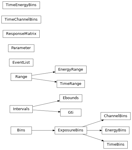
Class Inheritance Diagram