The Background Fitter (fitter)

Introduction

The BackgroundFitter class is an interface to binned and unbinned background fitting/estimation algorithms. Along with Polynomial and NaivePoisson, any fitting algorithm can be designed to be used with this interface by following the instructions for designing the classes for binned and unbinned data.

Examples

The first example is to fit a polynomial to some binned data. We can create and example Phaii object (see the Phaii example for more details):

>>> from gdt.core.data_primitives import TimeEnergyBins, Gti
>>> from gdt.core.phaii import Phaii
>>>
>>> counts = [[ 0,  0,  2,  1,  2,  0,  0,  0],
>>>           [ 3, 16, 10, 13, 14,  4,  3,  3],
>>>           [ 3, 23, 26, 13,  8,  8,  5,  5],
>>>           [ 4, 21, 19, 16, 13,  2,  3,  4],
>>>           [ 4, 20, 17, 11, 15,  2,  1,  5],
>>>           [ 6, 20, 19, 11, 11,  1,  4,  4]]
>>>
>>> tstart = [0.0000, 0.0039, 0.0640, 0.1280, 0.1920, 0.2560]
>>> tstop = [0.0039, 0.0640, 0.1280, 0.1920, 0.2560, 0.320]
>>> exposure = [0.0038, 0.0598, 0.0638, 0.0638, 0.0638, 0.0638]
>>> emin = [4.323754, 11.464164, 26.22962, 49.60019, 101.016815,
>>>         290.46063, 538.1436, 997.2431]
>>> emax = [11.464164, 26.22962, 49.60019, 101.016815, 290.46063,
>>>         538.1436, 997.2431, 2000.]
>>>
>>> data = TimeEnergyBins(counts, tstart, tstop, exposure, emin, emax)
>>> gti = Gti.from_list([(0.0000, 0.320)])
>>> phaii = Phaii.from_data(data, gti=gti, trigger_time=356223561.133346)

Now that we have some data, we can create the background fitter in the following way:

>>> from gdt.core.background.fitter import BackgroundFitter
>>> from gdt.core.background.binned import Polynomial
>>> fitter = BackgroundFitter.from_phaii(phaii, Polynomial)

This initializes the fitter and tells it that we are fitting binned data with the Polynomial algorithm. We then do the fit by passing any required algorithm-specific parameters:

>>> fitter.fit(order=1)

Here we are fitting a first-order polynomial. The fitting statistic and degrees-of-freedom of the fit can be retrieved:

>>> fitter.statistic
array([0.30476203, 0.94114281, 7.21404506, 0.9132082 , 4.56229056,
       3.42242964, 2.64862129, 0.51647908])
>>> fitter.dof
array([3., 3., 4., 4., 4., 3., 3., 3.])

Other properties can be retrieve (if defined), such as the fit statistic that is being used and any parameters passed to the fitter:

>>> fitter.statistic_name
'chisq'
>>> fitter.parameters
{'order': 1}

If you’re not happy with the fit, you can refit with different parameters. For example, we can fit a second order polynomial instead:

>>> fitter.fit(order=2)

Most importantly, you can interpolate the background model at any point:

>>> import numpy as np
>>> time_interp = np.linspace(0.0, 0.320, 21)
>>> back_rates = fitter.interpolate_bins(time_interp[:-1], time_interp[1:])
>>> back_rates
<BackgroundRates: 10 time bins;
 time range (0.0, 0.256);
 1 time segments;
 8 energy bins;
 energy range (4.323754, 2000.0);
 1 energy segments>

We define new time bin edges we want to interpolate over and it returns a BackgroundRates object containing the model background rates and uncertainty in each energy channel for each requested time bin. We can visually show this by creating a Lightcurve plot and adding the background to it (see Plotting Lightcurves for details):

>>> import matplotlib.pyplot as plt
>>> from gdt.core.plot.lightcurve import Lightcurve
>>> lcplot = Lightcurve(data=phaii.to_lightcurve(),
>>>                     background=back_rates.integrate_energy())
>>> plt.show()

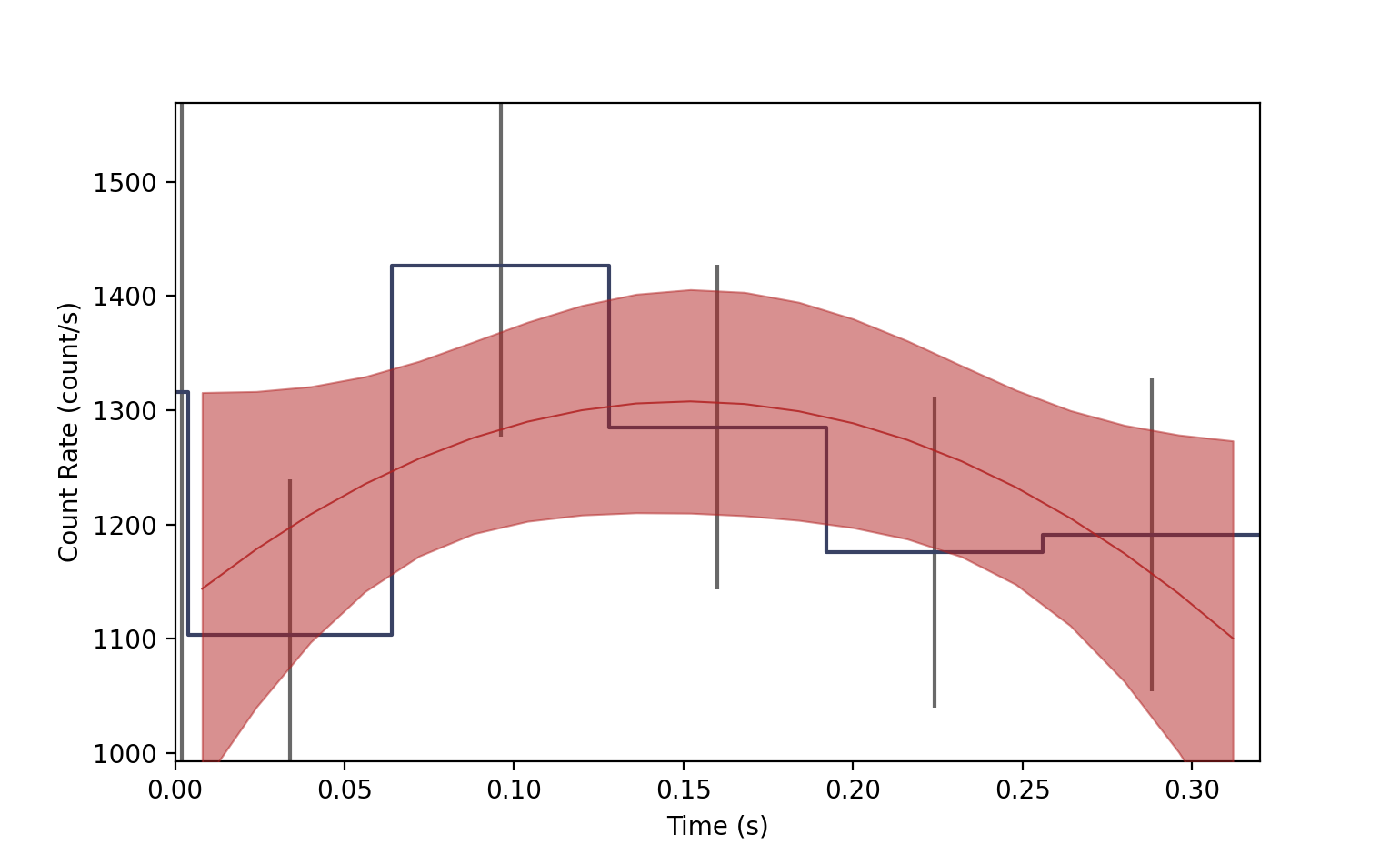
The blue bins are our lightcurve data with errorbars, and the background model is the red band, representing the 1-sigma uncertainty, and the model median line.

We can use BackgroundFitter in the same way to fit unbinned data. For example, let’s create some TTE data (see the PhotonList example for more details):

>>> from gdt.core.data_primitives import EventList, Ebounds, Gti
>>> # simulated Poisson rate of 1 count/sec
>>> times = np.random.exponential(1.0, size=100).cumsum()
>>> # random channel numbers
>>> channels = np.random.randint(0, 6, size=100)
>>> # channel-to-energy mapping
>>> ebounds = Ebounds.from_bounds([10.0, 20.0, 40.0, 80.0, 160.0, 320.0],
>>>                               [20.0, 40.0, 80.0, 160.0, 320.0, 640.0])
>>> data = EventList(times, channels, ebounds=ebounds)

>>> # construct the good time interval(s)
>>> gti = Gti.from_list([(0.0000, 100.0)])

>>> # create the PhotonList object
>>> from gdt.core.tte import PhotonList
>>> tte = PhotonList.from_data(data, gti=gti, trigger_time=356223561.,
>>>                            event_deadtime=0.001, overflow_deadtime=0.1)

Now, since we have TTE data, we can create our fitter this way:

>>> from gdt.core.background.unbinned import NaivePoisson
>>> fitter = BackgroundFitter.from_tte(tte, NaivePoisson)

And we can fit with the relevant algorithm parameters

>>> fitter.fit(window_width=10.0, fast=True)

Reference/API

gdt.core.background.fitter Module

Classes

BackgroundFitter()

Class for fitting a background, given a fitting algorithm, to time-energy data (e.g.

Class Inheritance Diagram