Spectral Functions (functions)

The spectral functions module provides both a base class for defining spectral functions that work within the GDT as well as a list of predefined spectral functions. The functionality of the base class supports spectral fitting and integration (flux) determination.

The Function Base Class

The Function class is the base class from which all GDT-provided and user-defined spectral functions are derived. It contains several attributes that are used to define default parameter values, allowable parameter ranges, and other attributes useful for spectral fitting. To illustrate these attributes, let’s initialize a simple power law function provided in the GDT:

>>> from gdt.core.spectra.functions import PowerLaw
>>> pl = PowerLaw()
>>> pl
<PowerLaw: 3 parameters;
 Defaults: A = 0.1 ph/s/cm^2/keV;
           index = -2.0 ;
           *Epiv = 100.0 >

The information printed here summarizes the default values for all of the parameters of the function and the * marks parameters which are fixed (i.e. are not considered free parameters).

To get the parameter list details, we access the param_list attribute:

>>> pl.param_list
[('A', 'ph/s/cm^2/keV', 'Amplitude'),
 ('index', '', 'Photon index'),
 ('Epiv', '', 'Pivot energy')]

This returns a list of tuples that tell us the parameter name, units of the parameter, and a short descriptor for that parameter.

We can also directly access the default parameter values and even update them if desired. We might want to update the defaults, for example, to initialize a spectral fit at a certain set of values instead of the defaults upon initialization.

>>> pl.default_values
[0.1, -2.0, 100.0]
>>> # update the default to be -1.5 for the index
>>> pl.default_values[1] = -1.5
>>> pl
<PowerLaw: 3 parameters;
 Defaults: A = 0.1 ph/s/cm^2/keV;
           index = -1.5 ;
           *Epiv = 100.0 >

Similarly, we can also retrieve and set which parameters are free and allowed for fitting:

>>> pl.free
[True, True, False]
>>> # fix the power law index
>>> pl.free[1] = False
>>> pl
<PowerLaw: 3 parameters;
 Defaults: A = 0.1 ph/s/cm^2/keV;
           *index = -1.5 ;
           *Epiv = 100.0 >

Other attributes that can be retrieved and set are the minimum and maximum allowed boundaries of the parameters (used by minimizers that place boundary constraints) and the maximum absolute and relative fitting step sizes (used by gradient descent algorithms).

>>> # minimum boundaries
>>> pl.min_values
[1e-10, -20.0, 0.01]

>>> # maximum boundaries
>>> pl.max_values
[inf, inf, inf]

>>> # max absolute step size
>>> pl.delta_abs
[0.1, 0.1, 0.1]

>>> # max relative step size
>>> pl.delta_rel
[0.01, 0.01, 0.01]

We can evaluate the function for a set of parameters (not necessarily the default values) by calling eval() with the parameter values and an array of energies at which to evaluate.

>>> import numpy as np
>>> # log-spaced array of size 10 from 10-1000 keV
>>> energies = np.geomspace(10.0, 1000.0, 10)
>>> # amplitude=0.05, index=-1.7; Epiv=100.0
>>> params = (0.05, -1.7, 100.0)
>>> pl.eval(params, energies)
array([2.50593617e+00, 1.05000708e+00, 4.39961272e-01, 1.84347253e-01,
       7.72429574e-02, 3.23654102e-02, 1.35613629e-02, 5.68231833e-03,
       2.38093633e-03, 9.97631157e-04])

That works well enough, but sometimes we don’t want to worry about defining a fixed value during the evaluation. If you want to use the fixed parameters at their default values without having to specify the parameter values upon evaluation, use fit_eval (so called because this is the function that is called when fitting):

>>> # assume Epiv is fixed at 100 and index is fixed at -1.5
>>> pl.fit_eval((0.05), energies)
array([1.58113883, 0.73389963, 0.34064603, 0.15811388, 0.07338996,
       0.0340646 , 0.01581139, 0.007339  , 0.00340646, 0.00158114])

Often we want to know what the photon or energy flux is for a given spectrum over a certain energy rain. We can easily integrate our spectrum and get out such a flux using the integrate() method. To do this, we need to provide the function parameters (can be all parameters or only the free parameters), define the energy range over which we will integrate, and specify if we integrating over the photon spectrum or the energy spectrum:

>>> # integrate over 50-300 keV to produce the photon flux (ph/cm^2/s)
>>> pl.integrate(params, (50.0, 300.0), energy=False)
8.293165460937157

>>> # integrate over 50-300 keV to produce the energy flux (erg/cm^2/s)
>>> pl.integrate(params, (50.0, 300.0), energy=True)
1.5436256788927548e-06

The SuperFunction Class

More complex functions can be made out of combinations of Function objects, specifically by adding or multiplying functions together. In this scenario, the combined function is treated as a SuperFunction, and the individual functions are treated as components of the SuperFunction.

As an example, let’s add a blackbody spectral function to our power law:

>>> from gdt.core.spectra.functions import BlackBody
>>> bb_pl = BlackBody() + PowerLaw()
>>> bb_pl
<BlackBody + PowerLaw: 5 parameters;
 Defaults: BlackBody: A = 0.01 ph/s/cm^2/keV;
           BlackBody: kT = 30.0 keV;
           PowerLaw: A = 0.1 ph/s/cm^2/keV;
           PowerLaw: index = -2.0 ;
           *PowerLaw: Epiv = 100.0 >

Our SuperFunction contains the two function components, and we can access all of the same attributes and methods as we can with a normal Function. One attribute to note is num_components, which tells us the number of spectral components contained in the SuperFunction.

Just like a normal Function, we can evaluate our SuperFunction:

>>> bb_params = (0.01, 15.0)
>>> pl_params = (0.05, -1.7)
>>> bb_pl.fit_eval(bb_params + pl_params, energies)
array([3.56108451e+00, 2.41358102e+00, 1.87592319e+00, 1.20667453e+00,
       4.22825011e-01, 6.27660049e-02, 1.38298600e-02, 5.68236914e-03,
       2.38093633e-03, 9.97631157e-04])

But with a SuperFunction, we now have the option of evaluating each component as well:

>>> bb_pl.fit_eval(bb_params + pl_params, energies, components=True)
[array([1.05514834e+00, 1.36357394e+00, 1.43596192e+00, 1.02232727e+00,
        3.45582054e-01, 3.04005947e-02, 2.68497101e-04, 5.08106585e-08,
        1.58018801e-14, 1.11438316e-25]),
 array([2.50593617e+00, 1.05000708e+00, 4.39961272e-01, 1.84347253e-01,
        7.72429574e-02, 3.23654102e-02, 1.35613629e-02, 5.68231833e-03,
        2.38093633e-03, 9.97631157e-04])]

This returns the function evaluation of each component in order (i.e. in our example the first array is the blackbody evaluation, then the power law evaluation).

And as an example, we can create a SuperFunction via multiplication:

>>> from gdt.core.spectra.functions import HighEnergyCutoff
>>> pl_cutoff = PowerLaw() * HighEnergyCutoff()
>>> pl_cutoff
<PowerLaw * HighEnergyCutoff: 5 parameters;
 Defaults: PowerLaw: A = 0.1 ph/s/cm^2/keV;
           PowerLaw: index = -2.0 ;
           *PowerLaw: Epiv = 100.0 ;
           HighEnergyCutoff: Ecut = 1000.0 keV;
           HighEnergyCutoff: EF = 100.0 keV>

For Developers:

Defining a new Function

To illustrate how to define a new spectral function, we will follow the design of the GDT-provided PowerLaw spectral function:

>>> import numpy as np
>>> from gdt.core.spectra.functions import Function
>>>
>>> class MyPowerLaw(Function):
>>>     nparams = 2 # this must be defined
>>>
>>>     # optional; will be filled with ambiguous defaults
>>>     param_list = [('A', 'ph/s/cm^2/keV', 'Amplitude'),
>>>                   ('index', '', 'Photon index'),
>>>                   ('Epiv', '', 'Pivot energy')]
>>>
>>>     # optional; although defaults will all be set to 1.0
>>>     default_values = [0.1, -2.0, 100.0]
>>>
>>>     # optional; default will be set to -np.inf
>>>     min_values = [1e-10, -20.0, 0.01]
>>>     # optional; default will be set to np.inf
>>>     max_values = [np.inf, np.inf, np.inf]
>>>
>>>     # optional; default will be set to 0.1
>>>     delta_abs = [0.1, 0.1, 0.1]
>>>     # optional; default will be set to 0.01
>>>     delta_rel = [0.01, 0.01, 0.01]
>>>
>>>     def eval(self, params, x):
>>>         # this must be defined as the function evaluation
>>>         # in our example, params is (A, index, Epiv)
>>>         return params[0] * (x / params[2]) ** params[1]

And if we instantiate it:

>>> MyPowerLaw()
<MyPowerLaw: 2 parameters;
 Defaults: A = 0.1 ph/s/cm^2/keV;
           index = -2.0 >

Reference/API

gdt.core.spectra.functions Module

Classes

Band()	The Band GRB function (a type of smoothly broken power law), parametrized by the peak of the \(\nu F_{\nu}\) spectrum:
BandOld()	The Band GRB function (a type of smoothly broken power law), using the original parameterization:
BlackBody()	Black Body spectrum:
BrokenPowerLaw()	A sharply-broken power law:
Comptonized()	An exponentially cut-off power law, parametrized by the peak of the \(\nu F_{\nu}\) spectrum:
DoubleBrokenPowerLaw()	A sharply-broken power law with two breaks:
GaussLine()	A Gaussian Line:
GaussLineMult()	A Gaussian Line (Multiplicative Component):
GaussianLog()	A Gaussian with \(log_{10}(E)\):
GaussianLogVaryingFWHM()	A Gaussian with \(log_{10}(E)\) and linearly-varying FWHM:
HighEnergyCutoff()	A High-Energy cutoff (Multiplicative Component):
LogNormal()	A Log-Normal function:
LorentzLineMult()	A Lorentzian Line (Multiplicative Component):
LowEnergyCutoff()	A Low-Energy cutoff (Multiplicative Component):
OTTB()	Optically-Thin Thermal Bremsstrahlung:
OTTS()	Optically-Thin Thermal Synchrotron:
PowerLaw()	A power law function:
PowerLawMult()	A Power Law (Multiplicative Component):
SmoothlyBrokenPowerLaw()	A smoothly-broken power law with a break scale:
SunyaevTitarchuk()	Sunyaev-Titarchuk Comptonization spectra:
TanakaPulsar()	Tanaka's pulsar model
YangSoongPulsar()	Yang Soong's pulsar spectral form
Function()	Abstract class for a 1-D function (e.g.
SuperFunction()	Abstract class for a sum or product of functions.

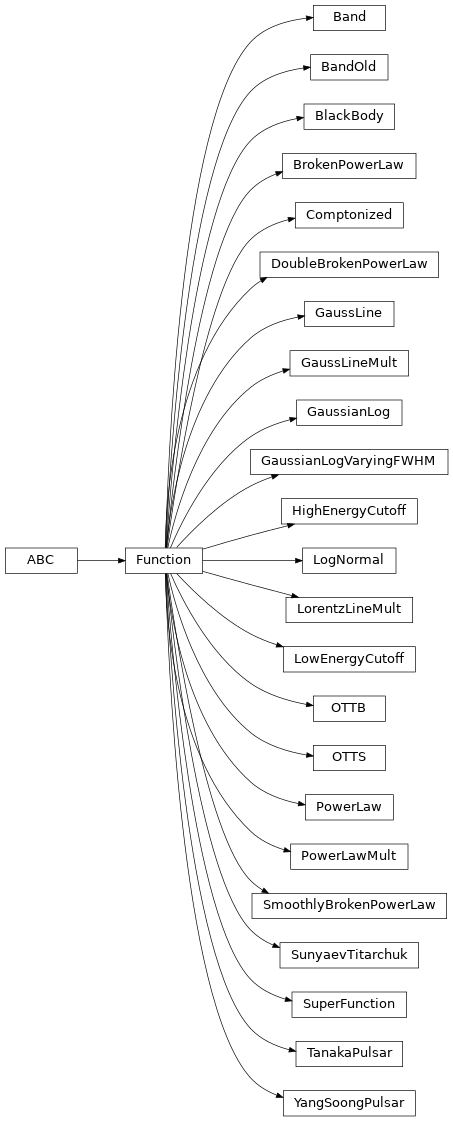
Class Inheritance Diagram