Instrument Responses (gdt.core.response)

Introduction

The instrument response for hard X-ray and gamma-ray detectors are generally represented as a matrix mapping the incident photon energy to the energy of the recorded _counts_. This matrix combines two primary factors: the effective area as a function of energy (which often includes other factors like efficiency), and the photon energy redistribution. A photon model can then be “folded” through this Detector Response Matrix (DRM) via matrix multiplication to produce the recorded counts in each detector energy channel. As a general rule, the DRM is not an invertible matrix because the energy redistribution causes the DRM to have significant off-diagonal contributions. This causes the matrix to be nearly singular and non-invertible. Even if the DRM could be inverted, data have statistical fluctuations so backing out a photon spectrum from a count spectrum will not work well.

A particular DRM is valid for a particular incidence direction. If multiple incidence directions are required for an analysis, then DRMs corresponding to those directions are needed. For example, in the case that the source-detector angle changes significantly during a time-resolved spectral analysis, it may be necessary to use a time series of DRMs. The GDT contains classes to work with single-DRM response files (Rsp) and multi-DRM response files (Rsp2).

The Rsp Class

The Rsp class provides a way to construct, write out, and read single-DRM response files. There are also some useful functions to rebin, resample, and fold a model through the response. The Rsp base class does not have the ability to read and write files. Rsp is expected to be subclassed to define the reading and writing portion of the file, however, you can still programmatically create a Rsp object. In the following examples, we will first create a Rsp object with a DRM, and then we will walk through how to subclass Rsp to create a class that can read/write files.

Examples

First, we will show how to construct a Rsp object from a DRM defined in a ResponseMatrix object. In our example, we will construct a response with a DRM that has 8 input photon bins and 4 output energy channels.

>>> from gdt.core.data_primitives import ResponseMatrix
>>> # 8 photon bins x 4 energy channels
>>> matrix = [[25.2,  0.0,  0.0,  0.0],
>>>           [51.8, 54.9,  0.0,  0.0],
>>>           [2.59, 82.0, 44.8,  0.0],
>>>           [3.10, 11.6, 77.0, 0.13],
>>>           [1.26, 6.21, 29.3, 14.6],
>>>           [0.45, 3.46, 13.8, 9.98],
>>>           [0.52, 4.39, 13.3, 3.93],
>>>           [0.79, 7.14, 16.1, 3.92]]
>>> emin = [5.00, 15.8, 50.0, 158., 500., 1581, 5000, 15811]
>>> emax = [15.8, 50.0, 158., 500., 1581, 5000, 15811, 50000]
>>> chanlo = [4.60, 27.3, 102., 538.]
>>> chanhi = [27.3, 102., 538., 2000]
>>> drm = ResponseMatrix(matrix, emin, emax, chanlo, chanhi)

>>> from gdt.core.response import Rsp
>>> tstart = 524666421.47
>>> tstop = 524666521.47
>>> trigtime = 524666471.47
>>> rsp = Rsp.from_data(drm, start_time=tstart, stop_time=tstop,
>>>                     trigger_time=trigtime, detector='det0')
>>> rsp
<Rsp:
trigger time: 524666471.47;
time range (-50.0, 50.0);
8 energy bins; 4 channels>

In this example, note that we constructed the Rsp object with a ResponseMatrix and some metadata, namely the the times over which the response is valid and a reference “trigger” time. While not required, it is strongly suggested that start_time and stop_time be defined, especially if this response is used in a time series analysis. And the detector name should be defined if this response is used in a multi-detector analysis.

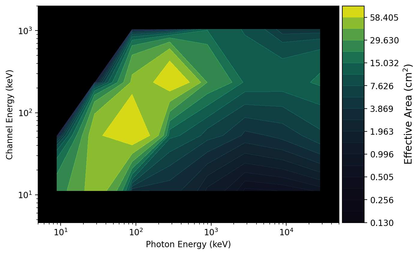
We can plot it to see what it looks like using the ResponsePlot class (see Response DRMs for details):

>>> import matplotlib.pyplot as plt
>>> from gdt.core.plot.drm import ResponsePlot
>>> drmplot = ResponsePlot(drm=rsp.drm, num_contours=20)
>>> plt.show()

Now that we have created our Rsp object, there are several attributes that are available to us. We can directly access the DRM and times we created the object with:

>>> # the DRM
>>> rsp.drm
<ResponseMatrix: 8 energy bins; 4 channels>
>>> # start time
>>> rsp.tstart
-50.0
>>> # stop time
>>> rsp.tstop
50.0
>>> # reference time
>>> rsp.trigtime
524666471.47
>>> rsp.detector
'det0'

There are other attributes that are exposed:

>>> # the energy channel ebounds
>>> rsp.ebounds
<Ebounds: 4 intervals; range (4.6, 2000.0)>
>>> # number of energy channels
>>> rsp.num_chans
4
>>> # number of photon bins
>>> rsp.num_ebins
8
>>> # center of valid time interval
>>> rsp.tcent
0.0

The single most important function of the Rsp object is the ability to fold a photon spectrum through the response and get out a count rate. While the lower-level ResponseMatrix object does the heavy lifting of the folding, the Rsp object formats the output into an EnergyBins object containing a count rate spectrum and incorporating an exposure. In our example, we will use the built-in PowerLaw function to fold a -2.2 power law through the response matrix:

>>> from gdt.core.spectra.functions import PowerLaw
>>> pl = PowerLaw()
>>> # amplitude = 0.01; index = -2.2; 2.5 s exposure
>>> count_spectrum = rsp.fold_spectrum(pl.fit_eval, (0.01, -2.2), exposure=2.5)
>>> count_spectrum
<EnergyBins: 4 bins;
range (4.6, 2000.0);
2 contiguous segments>
>>> count_spectrum.rates
array([852.91654884, 425.86251321,  92.80740883,   1.58433796])

Other functions include rebinning energy channel axis and resampling the the input photon axis of the response. You can rebin the energy channel axis in two ways: either by specifying a binning factor at which to downscale the axis resolution (e.g. a rebinning factor of 2 combines the energy channels by a factor of two) or by specifying the energy channel edges that should remain in the rebinned axis.

>>> # rebin by a factor of 2
>>> rebinned_rsp = rsp.rebin(factor=2)
>>> rebinned_rsp.ebounds.intervals
[<EnergyRange: (4.6, 102.0)>,
<EnergyRange: (102.0, 2000.0)>]

>>> # rebin by only showing the specified edges (defined by edge index)
>>> rebinned_rsp = rsp.rebin(edge_indices=[0, 1, 2, 4])
>>> rebinned_rsp.ebounds.intervals
[<EnergyRange: (4.6, 27.3)>,
<EnergyRange: (27.3, 102.0)>,
<EnergyRange: (102.0, 2000.0)>]

Resampling the input axis of the response allows a lot more flexibility; you can increase the resolution of the input axis, decrease the resolution, or just redefine the energy edges as long as the edges are still contained within the bounds of the original response. This can all be done with two options: specifying the number in input photon bins, or specifying the photon bin edges. If you specify the number of photon bins, they will be logarithmically spaced between the bounds of the original response.

>>> # resample by specifying 10 logarithmically-spaced bins
>>> resampled_rsp = rsp.resample(num_photon_bins=10)
>>> resampled_rsp.drm.photon_bins.intervals
[<EnergyRange: (5.000000000000001, 12.559432157547903)>,
<EnergyRange: (12.559432157547903, 31.54786722400968)>,
<EnergyRange: (31.54786722400968, 79.2446596230557)>,
<EnergyRange: (79.2446596230557, 199.05358527674863)>,
<EnergyRange: (199.05358527674863, 499.99999999999994)>,
<EnergyRange: (499.99999999999994, 1255.943215754791)>,
<EnergyRange: (1255.943215754791, 3154.786722400968)>,
<EnergyRange: (3154.786722400968, 7924.4659623055695)>,
<EnergyRange: (7924.4659623055695, 19905.358527674885)>,
<EnergyRange: (19905.358527674885, 49999.99999999999)>]

>>> # resample by specifying the photon bin edges
>>> resampled_rsp = rsp.resample(photon_bin_edges=[5.0, 50.0, 500.0, 5000., 50000.])
>>> resampled_rsp.drm.photon_bins.intervals
[<EnergyRange: (5.0, 50.0)>,
<EnergyRange: (50.0, 500.0)>,
<EnergyRange: (500.0, 5000.0)>,
<EnergyRange: (5000.0, 50000.0)>]

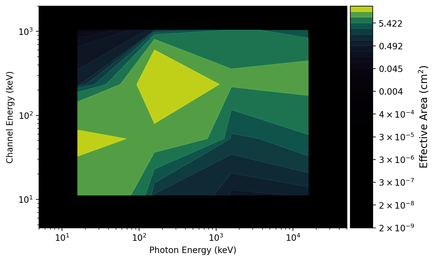
The plot of the second resampled DRM is shown below:

>>> drmplot = ResponsePlot(drm=resampled_rsp.drm, num_contours=40)
>>> plt.show()

For Developers:

Subclassing

To read and write single-DRM RSP files, the Rsp class needs to be subclassed. This is because the format and metadata of the files can be different from mission to mission. When subclassing Rsp to read a file, the open() method needs to be defined. To write out a file, the private method _build_hdulist() needs to be defined, which defines the data structure for each extension of the FITS file. Adding header information/metadata is not required, however if you do want the header information to be tracked when reading in a file and written out when writing a file to disk, you will need to create the header definitions as explained in Data File Headers and also define the private method _build_headers().

To illustrate further, below is a sketch of how the Rsp class should be subclassed in the example MyRsp:

>>> import astropy.io.fits as fits
>>> from gdt.core.data_primitives import ResponseMatrix
>>> from gdt.core.response import Rsp
>>>
>>> class MyRsp(Rsp):
>>>     """An example to read and write Rsp files for xxx instrument"""
>>>     @classmethod
>>>     def open(cls, file_path, **kwargs):
>>>         with super().open(file_path, **kwargs) as obj:
>>>
>>>             # an example of how to set the headers
>>>             hdrs = [hdu.header for hdu in obj.hdulist]
>>>             headers = MyFileHeaders.from_headers(hdrs)
>>>
>>>             # an example of how to set the DRM
>>>             # Note: Some DRMs may be stored in a compressed format.
>>>             #       You will need to perform the decompression.
>>>             drm = ResponseMatrix(matrix, emin, emax, chan_lo, chan_hi)
>>>
>>>             return cls.from_data(drm, start_time=tstart, stop_time=tstop,
>>>                                  trigger_time=trigger_time,
>>>                                  filename=obj.filename, headers=headers)
>>>
>>>     def _build_hdulist(self):
>>>         # this is where we build the HDU list (header/data for each extension)
>>>         hdulist = fits.HDUList()
>>>
>>>         # some code to create PRIMARY HDU
>>>         # ...
>>>         hdulist.append(primary_hdu)
>>>
>>>         # code to create other HDUs and append to hdulist
>>>         # ...
>>>
>>>         return hdulist
>>>
>>>     def _build_headers(self, num_chans, num_ebins):
>>>         # build the header based on these inputs
>>>         headers = self.headers.copy()
>>>         # update header information here
>>>         # ...
>>>
>>>         return headers

To create a Rsp object from a FITS file, the open() method should, at a minimum, be able to construct a ResponseMatrix object containing the DRM. Additionally, you can construct a FileHeaders and define the relevant time range. If the data has an associated trigger or reference time, you can track that as well.

The example creation of headers takes in a list of the headers from each extension and assumes you have created a class (in this case MyFileHeaders) that will read in the header information.

To write the data to disk, the _build_hdulist() defines the list of FITS HDUs, and is called by the write() method. The _build_headers() method is called whenever operations are performed on the object, like rebinning or slicing to propagate the header information.

The Rsp2 Class

Often it is useful to write several DRMs, in a time sequence, to a single file. For analyses that require studying the spectrum on a timescale over which the instrument pointing relative to the source in consideration has changed, then a different DRM may be needed for different time segments of the analysis. For this purpose, RSP2 files contain two or more DRMs that are each associated with a GTI. An analysis can then use the appropriate DRM, or weigh the different DRMs based on the time interval(s) of interest. The Rsp2 class provides the functionality for creating, reading, and writing RSP2 files and extracting individual DRMs, interpolating DRMs, and weighting DRMs.

Examples

For simplicity, let’s use the DRM we defined above and simply create two more DRMs that are just scalar increases from the original:

>>> import numpy as np
>>> matrix = np.copy(drm.matrix)
>>> drm_2 = ResponseMatrix(matrix*1.1, emin, emax, chanlo, chanhi)
>>> drm_3 = ResponseMatrix(matrix*1.2, emin, emax, chanlo, chanhi)

Now we create the response objects with the GTI for each response

>>> rsp_2 = Rsp.from_data(drm_2, start_time=tstart+100.0, stop_time=tstop+100.0,
>>>                       trigger_time=trigtime)
>>> rsp_3 = Rsp.from_data(drm_3, start_time=tstart+200.0, stop_time=tstop+200.0,
>>>                       trigger_time=trigtime)

Now we can create a Rsp2 object from these three responses:

>>> from gdt.core.response import Rsp2
>>> rsp2 = Rsp2.from_rsps([rsp, rsp_2, rsp_3])
>>> rsp2
<Rsp2:
 trigger time: 524666471.47; 3 DRMs;
 time range (-50.0, 250.0)>

Once created, we can retrieve the Ebounds that is common to all the DRMs, as well as the number of channels, number of energy bins, and number of DRMs:

>>> rsp2.ebounds
<Ebounds: 4 intervals; range (4.6, 2000.0)>

>>> rsp2.num_chans
4

>>> rsp2.num_ebins
8

>>> rsp2.num_drms
3

We can also retrieve the times over which each DRM can be used:

>>> rsp2.tstart
array([-50.,  50., 150.])

>>> rsp2.tstop
array([ 50., 150., 250.])

>>> rsp2.tcent
array([  0., 100., 200.])

Each individual DRM can be extracted in a number of ways. The Rsp2 object is indexed, which means that we can retrieve each individual response by index:

>>> rsp2[1]
<Rsp:
 trigger time: 524666471.47;
 time range (50.0, 150.0);
 8 energy bins; 4 channels>

You can also use extract_drm() to return individual responses by index or by time:

>>> rsp2.extract_drm(index=0)
<Rsp:
 trigger time: 524666471.47;
 time range (-50.0, 50.0);
 8 energy bins; 4 channels>

>>> # get the response for T0+175.0
>>> rsp2.extract_drm(atime=175.0)
<Rsp:
 trigger time: 524666471.47;
 time range (150.0, 250.0);
 8 energy bins; 4 channels>

Instead of simply extracting an existing response, we can interpolate using our current list of responses and return a new response:

>>> # interpolate at T0+175
>>> rsp2.interpolate(atime=175.0)
<Rsp:
 trigger time: 524666471.47;
 time range (175.0, 175.0);
 8 energy bins; 4 channels>

An alternative, especially for long-duration time-integrated analysis, is to generate a weighted response. This is done by providing a time history of observed counts (lightcurve) which is used to weight each appropriate DRM, and then the sum of the weighted DRMs are provided in a new response object.

As an example, let us consider that we have 20 s time bins containing counts from T0 to T0+200 s.

>>> from gdt.core.data_primitives import TimeBins
>>> times = np.linspace(0.0, 200.0, 11)
>>> counts = [100, 110, 90, 150, 220, 70, 50, 140, 410, 230]
>>> exposure = [19.9]*10
>>> bins = TimeBins(counts, times[:-1], times[1:], exposure)
>>> bins
<TimeBins: 10 bins;
 range (0.0, 200.0);
 1 contiguous segments>

Now we use this to create a weighted response. We can choose to use interpolation when weighting, too.

>>> weighted1 = rsp2.weighted(bins, interpolate=False)
>>> weighted1.drm.matrix
array([[28.77936306,  0.        ,  0.        ,  0.        ],
       [59.15757962, 62.69789809,  0.        ,  0.        ],
       [ 2.95787898, 93.64713376, 51.1633121 ,  0.        ],
       [ 3.54031847, 13.24764331, 87.93694268,  0.14846497],
       [ 1.43896815,  7.09205732, 33.46171975, 16.67375796],
       [ 0.5139172 ,  3.95145223, 15.76012739, 11.3975414 ],
       [ 0.59385987,  5.01354777, 15.18910828,  4.48821019],
       [ 0.90221019,  8.15415287, 18.38681529,  4.47678981]])

>>> weighted2 = rsp2.weighted(bins, interpolate=True)
>>> weighted2.drm.matrix
array([[28.21276433,  0.        ,  0.        ,  0.        ],
       [57.99290446, 61.46352229,  0.        ,  0.        ],
       [ 2.89964522, 91.80343949, 50.15602548,  0.        ],
       [ 3.47061783, 12.98682803, 86.20566879,  0.14554204],
       [ 1.41063822,  6.95243121, 32.80293631, 16.34549045],
       [ 0.50379936,  3.87365732, 15.44984713, 11.17315032],
       [ 0.58216815,  4.91484268, 14.89007006,  4.39984777],
       [ 0.88444777,  7.99361656, 18.02482166,  4.38865223]])

Reference/API

gdt.core.response Module

Classes

Rsp()	Class for single-DRM responses.
Rsp2()	Class for multiple-DRM responses.

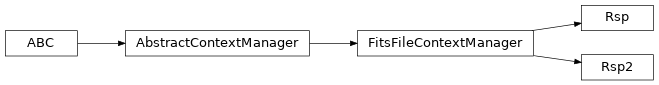
Class Inheritance Diagram

Special Methods

Rsp._build_hdulist()

This builds the HDU list for the FITS file. This method needs to be specified in the inherited class. The method should construct each HDU (PRIMARY, EBOUNDS, SPECTRUM, GTI, etc.) containing the respective header and data. The HDUs should then be inserted into a HDUList and that list returned

Returns:

(astropy.io.fits.HDUList)

Rsp._build_headers(num_chans, num_ebins)

This builds the headers for the FITS file. This method needs to be specified in the inherited class. The method should construct the headers from the minimum required arguments and additional keywords and return a FileHeaders object.

Parameters:

• num_chans (int) – Number of detector energy channels

• num_ebins (int) – Number of photon energy bins

Returns:

(FileHeaders)