Simulating PHA Spectral Data (pha)

This module enables the simulation of spectral data including mixtures of background and source, which is handled by PhaSimulator.

For source simulation, a detector response and photon model are required as the photon model must be folded through the response to produce a count spectrum. That count spectrum is then sampled from to produce Poisson deviates of the count spectrum.

Because folding an inherent photon/particle spectrum through the full-sky response and integrating over the sky is a very complex and fraught process, the background simulation is handled in a different way. The simulator assumes that you already have some estimate of the background count spectrum. This can either be produced directly from real background data, derived (fit) to real background data, or created manually. The input background spectrum is then used to produce Poisson or Gaussian deviates of the background.

As an example to demonstrate how to produce such simulations, we will use the example detector response constructed in The Rsp Class, and then we will use a Band function (see Spectral Functions for more information on photon models). For the input background spectrum, we must provide a BackgroundSpectrum object, which we will manually create in this example:

>>> from gdt.core.background.primitives import BackgroundSpectrum
>>> rates = [37.5, 57.5, 17.5, 27.5]
>>> rate_uncert = [1.896, 2.889, 0.919, 1.66]
>>> emin = [4.60, 27.3, 102., 538.]
>>> emax = [27.3, 102., 538., 2000]
>>> exposure = 0.256
>>> back_spec = BackgroundSpectrum(rates, rate_uncert, emin, emax, exposure)

Now we are set to initialize our PHA simulator:

>>> from gdt.core.simulate.pha import PhaSimulator
>>> from gdt.core.spectra.functions import Band
>>> band_params = (0.01, 300.0, -1.0, -2.8)
>>> sim = PhaSimulator(rsp, Band(), band_params, 0.256, back_spec, 'Gaussian')

Here, we specified our detector response (rsp), the spectral function and parameters, the exposure (0.256), the background spectrum, and the distribution from which to draw background deviates (either 'Gaussian' or 'Poisson')

Note

The exposure on initialization of PhaSimulator does NOT have to match the exposure in the BackgroundSpectrum. The BackgroundSpectrum will be scaled to the corresponding exposure used in the simulations.

Now we can generate deviates of the source signal in the following way:

>>> source_devs = sim.simulate_source(20)
>>> source_devs[0]
<EnergyBins: 4 bins;
 range (4.6, 2000.0);
 1 contiguous segments>

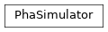
In the above, we generated 20 Poisson deviates of the source spectrum, which are packaged in EnergyBins objects. To visualize what these deviates look like, we can plot them using the Spectrum plotting class and Histo plotting elements (see Plotting Count Spectras for more information).

>>> import matplotlib.pyplot as plt
>>> from gdt.core.plot.spectrum import Spectrum
>>> from gdt.core.plot.plot import Histo
>>> # initialize
>>> specplot = Spectrum()
>>> # add each deviate to the plot
>>> source_dev_plt = [Histo(source_dev, specplot.ax, color='midnightblue',
>>>                   alpha=0.2) for source_dev in source_devs]
>>> plt.show()

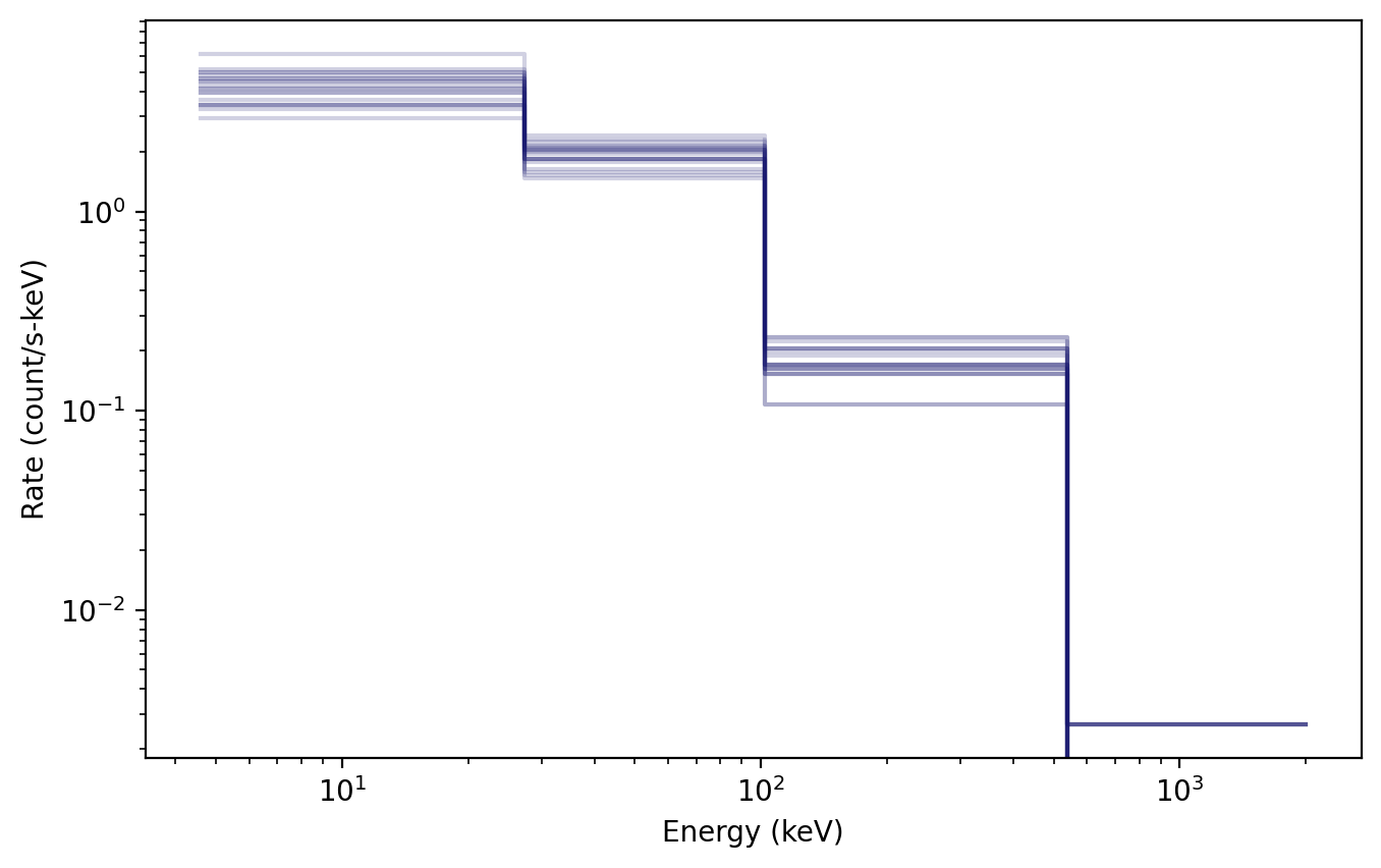
We can also generate deviates of the background in a similar manner:

>>> bkgd_devs = sim.simulate_background(20)
>>> bkgd_devs[0]
<BackgroundSpectrum: 4 bins;
 range (4.6, 2000.0);
 1 contiguous segments>

This can also plotted using the SpectrumBackground plot element:

>>> from gdt.core.plot.plot import SpectrumBackground
>>> specplot = Spectrum()
>>> bkgd_dev_plt = [SpectrumBackground(bkgd_dev, specplot.ax, color='gray',
>>>                 alpha=0.1, band_alpha=0.05) for bkgd_dev in bkgd_devs]
>>> plt.show()

Of most use is to combine the background and source together to create deviates of the observed spectrum, which are, again, returned as EnergyBins objects.

>>> sum_devs = sim.simulate_sum(20)
>>> sum_devs[0]
<EnergyBins: 4 bins;
 range (4.6, 2000.0);
 1 contiguous segments>

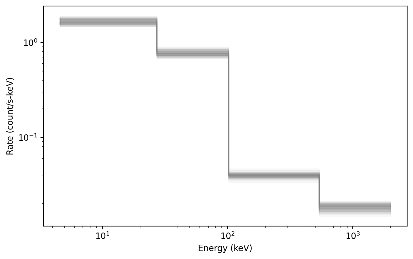
A particularly useful plot is to show the total spectral deviates and the background spectral deviates, which basically combines the plot commands from earlier:

>>> specplot = Spectrum()
>>> bkgd_dev_plt = [SpectrumBackground(bkgd_dev, specplot.ax, color='gray',
>>>                 alpha=0.1, band_alpha=0.05) for bkgd_dev in bkgd_devs]
>>> sum_dev_plt = [Histo(sum_dev, specplot.ax, color='midnightblue',
>>>                alpha=0.2) for sum_dev in sum_devs]
>>> plt.show()

As can be seen in the plot, the total observed spectral deviates are clearly above the background in all but the last energy channel, which indicates the signal is too weak to be distinguished from background in the last channel.

In addition to generating the deviates in GDT-native objects, the background deviates can be generated into Bak objects, and the total observed spectrum can be generated into Pha objects so that they can be written to file to be used in external analyses:

>>> sim.to_bak(1)
[<Bak:
  time range (0.0, 0.256);
  energy range (4.6, 2000.0)>]

>>> sim.to_pha(1)
[<Pha:
  time range (0.0, 0.256);
  energy range (4.6, 2000.0)>]

We can also concatenate a series of observed spectral deviates into a time-series Phaii object, which can also be written to file:

>>> phaii = sim.to_phaii(100)
>>> phaii
<Phaii:
 time range (0.0, 25.6);
 energy range (4.6, 2000.0)>

We can plot the energy-integrated “lightcurve” of these simulations using the Lightcurve plotting class:

>>> from gdt.core.plot.lightcurve import Lightcurve
>>> lcplot = Lightcurve(phaii.to_lightcurve())
>>> plt.show()

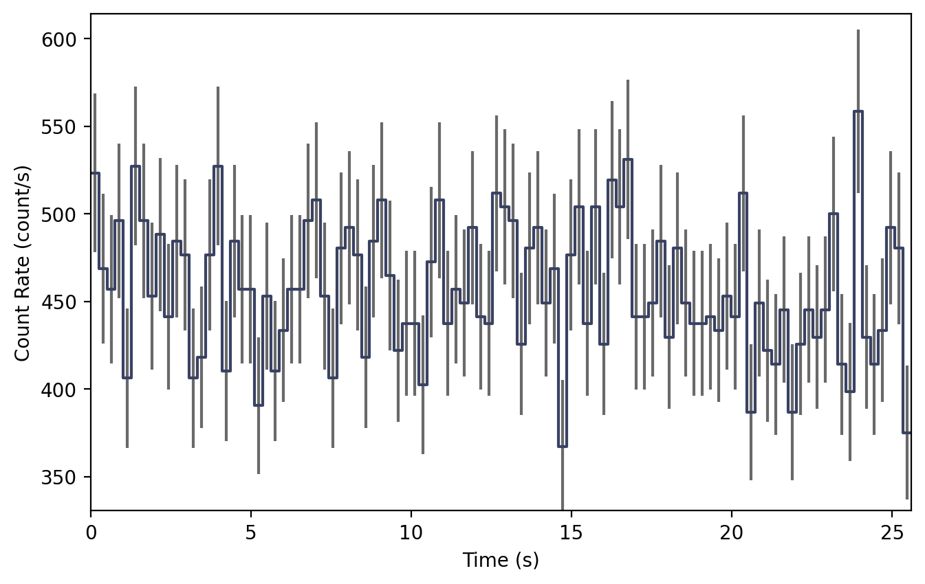
Note that each bin of this “lightcurve” corresponds to a single spectral deviate, and so the variation seen results from the Poisson variance of the source spectrum as well as the Poisson/Gaussian variance of the background spectrum.

Once initialized, the background, response, and source spectrum can be updated using set_background(), set_rsp(), and set_source(), respectively.

Seeding PHA Data

Users can set the random generator used to create each simulation with the rng keyword when initializing the PhaSimulator class:

>>> import numpy as np
>>> rng = np.random.default_rng(seed=1)
>>> sim = PhaSimulator(rsp, Band(), band_params, 0.256, back_spec, 'Gaussian', rng=rng)

This is useful in cases where reproducibility with a known seed is desired, such as for publicly shared simulation results.

Additionally, the random generator can be modified after initialization with the set_rng() function:

>>> sim.set_rng(rng)

In cases where the user does not provide their own generator, PhaSimulator uses np.random.default_rng() to create a default generator seeded by the computer’s clock time. This default generator will produce a different result whenever the simulation is performed at a different time. Simulations run at the same time will produce the same result, which can be problematic for users trying to run simulations as parallel processes. To avoid this, users should provide unique seeds to each simulation process when running in parallel. Below is an example of this for two parallel processes launched within a main function using Python’s multiprocessing module:

>>> import numpy as np
>>> import multiprocessing
>>>
>>> from gdt.core.data_primitives import ResponseMatrix
>>> from gdt.core.response import Rsp
>>> from gdt.core.background.primitives import BackgroundSpectrum
>>> from gdt.core.simulate.pha import PhaSimulator
>>> from gdt.core.spectra.functions import Band
>>>
>>> def simulate(proc_id: int, n: int, rng: np.random.Generator, results: dict, sim: PhaSimulator):
>>>     sim.set_rng(rng)
>>>     results[proc_id] = sim.simulate_source(n)
>>>
>>> if __name__ == "__main__":
>>>
>>>     rsp = ...
>>>     back_spec = ...
>>>     band_params = ...
>>>
>>>     sim = PhaSimulator(rsp, Band(), band_params, 0.256, back_spec, 'Gaussian')
>>>
>>>     manager = multiprocessing.Manager()
>>>     results = manager.dict()
>>>
>>>     # perform 20 simulations split across 2 parallel processes
>>>     rngs = np.random.default_rng().spawn(2)
>>>     procs = [multiprocessing.Process(target=simulate, args=(i, 10, rng, results, sim))
>>>              for i, rng in enumerate(rngs)]
>>>     [proc.start() for proc in procs]
>>>     [proc.join() for proc in procs]
>>>
>>>     for proc_id in sorted(results.keys()):
>>>         print(proc_id, results[proc_id])

Note that this requires the simulate() target method to be defined outside the main scope. Users looking for more flexibility or the ability to perform parallel processing within a Notebook should consider using the multiprocess dependency instead. This dependency is an extension of mulitprocessing that allows Manager() and Process() to be used in more scenarios, including within Notebooks.

Reference/API

gdt.core.simulate.pha Module

Classes

PhaSimulator(rsp, function, params, ...[, rng])

Simulate PHA data given a modeled background spectrum, detector response, source spectrum, and exposure.

Class Inheritance Diagram