Fermi GBM Position/Attitude History Data (gdt.missions.fermi.gbm.poshist)

Probably the most critical auxiliary file GBM produces is the position history (POSHIST) file. The POSHIST contains, for an entire day, the spacecraft location in orbit and pointing information, sampled on a 1 second timescale. If you are just interested in triggered GRB analysis where all of the response files are already made for you, then POSHIST may not be of much interest. But if you are using the continuous data in any way, the POSHIST is your dearest friend. You may want to know if a source is visible at a particular time (i.e. not behind the Earth), and if it is, what is the closest detector to the source. You may want to know if there are specific contributions to the background during a time interval, such as sun visibility or high geomagnetic latitude in orbit. You may want to rotate something from the equatorial frame to the Fermi inertial frame, or vice versa. Or you may want to make a pretty gif of the detector pointings over time.

To read a POSHIST file, we open it with the GbmPosHist class:

>>> from gdt.core import data_path
>>> from gdt.missions.fermi.gbm.poshist import GbmPosHist
>>> filepath = data_path.joinpath('fermi-gbm/glg_poshist_all_170101_v01.fit')
>>> poshist = GbmPosHist.open(filepath)
>>> poshist
<GbmPosHist(filename="glg_poshist_all_170101_v01.fit") at 0x12b372640>

The poshist object contains the spacecraft frame, which is the spacecraft position and orientation as a function of time, and the spacecraft states, which are the series of state flags as a function of time.

To see what state flags are available, we can retrieve the spacecraft states in the following way:

>>> states = poshist.get_spacecraft_states()
>>> states
<TimeSeries length=86520>
      time       sun   saa  good
      Time       bool  bool bool
---------------- ---- ----- ----
504921545.740106 True False True
504921546.740107 True False True
504921547.740107 True False True
504921548.740106 True False True
             ...  ...   ...  ...
505008060.340076 True False True
505008061.340078 True False True
505008062.340075 True False True
505008063.340076 True False True
505008064.340076 True False True

The state flags are stored in an Astropy TimeSeries object, and for each sampled time, there is a flag denoting if the sun is visible, if the spacecraft is in SAA, and if the data are in a good time interval (which in this case is just the opposite of the SAA flag).

We can, for example create a Good Time Intervals Gti object from the time and good columns:

>>> from gdt.core.data_primitives import Gti
>>> gti = Gti.from_boolean_mask(states['time'].value, states['good'].value)
>>> gti
<Gti: 10 intervals; range (504921545.740106, 505008064.340076)>

Regarding the spacecraft frame, we can retrieve it as a SpacecraftFrame object:

>>> frame = poshist.get_spacecraft_frame()
<SpacecraftFrame: 86520 frames;
 obstime=[504921545.740106, ...]
 obsgeoloc=[(-6315714., -1549390.6, 2302684.5) m, ...]
 obsgeovel=[(1011.3916, -7244.9014, -2100.9446) m / s, ...]
 quaternion=[(x, y, z, w) [-0.21889446,  0.00818764,  0.65160715, -0.72624121], ...]>

You will notice that this frame has a location in Earth Inertial Coordinates (obsgeoloc), the velocity of the spacecraft with reference to the Earth Inertial Coordinate frame (obsgeovel), and the spacecraft orientation quaternion, each for a given time stamp (obstime).

Let’s say we are interested in data around a specific time, for example MET=504975500. We can generate an interpolated frame at the requested time, as long as it exists within the boundaries of the file.

>>> from gdt.missions.fermi.time import *
>>> time = Time(504975500, format='fermi')
>>> one_frame = frame.at(time)
>>> one_frame
<SpacecraftFrame: 1 frames;
 obstime=[504975500.0]
 obsgeoloc=[(6294771.65990569, -825118.18949373, -2751704.74152787) m]
 obsgeovel=[(1531.48673123, 7317.65930685, 1296.24008645) m / s]
 quaternion=[(x, y, z, w) [ 0.20026199, -0.66690538,  0.49459807, -0.52010105]]>

We can retrieve where Fermi was in orbit at that time:

>>> one_frame.earth_location.lat, one_frame.earth_location.lon
(<Latitude -23.46926302 deg>, <Longitude 26.7365118 deg>)
>>>one_frame.earth_location.height
<Quantity 544542.2936586 m>)

We might be interested to know where the Earth is (and its apparent radius) relative to Fermi:

>>> one_frame.geocenter.ra, one_frame.geocenter.dec
(<Longitude 172.53224953 deg>, <Latitude 23.43352709 deg>)

>>> one_frame.earth_angular_radius
<Quantity 67.1226193 deg>

We could also be interested in a particular known source, and it would be helpful to know if it is even visible to Fermi at the time of interest:

>>> from astropy.coordinates import SkyCoord
>>> coord = SkyCoord(324.3, -20.8, frame='icrs', unit='deg')
>>> one_frame.location_visible(coord)
True

Well, that’s good to know. But we want to look at the data for the closest detector to that position. We can figure that out. For example, we can determine the angle between the ‘n0’ detector and that position on the sky:

>>> one_frame.detector_angle('n0', coord)
<Angle [4.27219806] deg>

Sometimes it’s useful to transform a source location of interest in equatorial coordinates to the Fermi inertial frame. You can do that by the following:

>>> coord_sc_frame = coord.transform_to(one_frame)
>>> coord_sc_frame.az, coord_sc_frame.el
(<Longitude [39.67934005] deg>, <Latitude [65.85535956] deg>)

Note that the frame transformation is in azimuth and elevation. It’s important to note that the Fermi inertial frame is defined by azimuth (0-360 deg) and elevation (-90-90 deg) or zenith (0-180 deg). Here, azimuth=0 is approximately the pointing of detector NaI 5, and increases counter-clockwise when looking down the LAT boresight. Elevation=90 (zenith=0) is defined as the LAT boresight, and elevation=-90 (zenith=180) is directly below the spacecraft.

You can also go from Fermi (azimuth, elevation) coordinates to equatorial coordinates:

>>> # Az=0, El=90 (the Fermi LAT boresight)
>>> sc_coord = SkyCoord(0.0, 90.0, frame=one_frame, unit='deg')
>>> sc_coord.icrs
<SkyCoord (ICRS): (ra, dec) in deg
    [(333.15399016, 1.73430464)]>

Note that any and all of these operations can be performed on an array of frames, even on the entire series of frames contained within the poshist file. For more details on working with the SpacecraftFrame, see Spacecraft Attitude, Position, and Coordinates.

Now all of this great, but we can also make a sky plot at a given time. We can plot in either the Equatorial frame:

>>> import matplotlib.pyplot as plt
>>> from gdt.core.plot.sky import EquatorialPlot
>>> eqplot = EquatorialPlot()
>>> eqplot.add_frame(one_frame)
>>> plt.show()

Or the Galactic Frame:

>>> from gdt.core.plot.sky import GalacticPlot
>>> galplot = GalacticPlot()
>>> galplot.add_frame(one_frame)
>>> plt.show()

Or the Spacecraft Frame:

>>> from gdt.core.plot.sky import SpacecraftPlot
>>> scplot = SpacecraftPlot()
>>> scplot.add_frame(one_frame)
>>> plt.show()

See Plotting Sky Maps, Localizations, and Wide-field Effective Area for more details on these plots.

Finally, we can plot a segment of the Fermi orbit and the location of Fermi at our desired time:

>>> from gdt.missions.fermi.plot import FermiEarthPlot
>>> from gdt.missions.fermi.gbm.saa import GbmSaa
>>> earthplot = FermiEarthPlot(saa=GbmSaa())
>>> # orbit segment 1000 s prior to our time of interest and 1000 s after
>>> earthplot.add_spacecraft_frame(frame, tstart=Time(time.fermi-1000, format='fermi'),
>>>                                tstop=2000, trigtime=time)
>>> earthplot.standard_title()
>>> plt.show()

Reference/API

gdt.missions.fermi.gbm.poshist Module

Classes

GbmPosHist()

Class for reading a GBM Position history file, which contains the spacecraft position, attitude (orientation), velocity, and various state information.

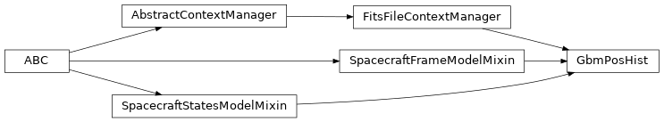
Class Inheritance Diagram