Simulating Event Data (tte)

This module contains two classes for simulating background and source event data: TteBackgroundSimulator and TteSourceSimulator, respectively. Unlike the PHA simulations, these event simulations contain a full temporal-spectral simulation given source/background spectra and temporal profiles.

Similar to PhaSimulator, these simulations rely on the underlying spectral shape; however, simulating event data allows the amplitude of the spectrum to change according to a temporal profile. The temporal profile could be as simple as a constant background and a tophat-shaped signal or as complex as a high order polynomial background and a parametric pulse shape. The simulation process first draws deviates from the spectrum to determine the count rate in each energy channel during a small slice of time (a sampling period). The number of counts in each channel is determined from the duration of the sampling period, and then arrival times are simulated for the events based on an exponential distribution. The duration of the sampling period for the event simulation is considered the timescale above which the generated events are indistinguishable from a non-stationary Poisson process. For example, if we wish to simulate a signal with temporal structure exhibited on 1 ms timescales, then we should choose a sampling period of < 1 ms.

An additional parameter in the event data simulators is the deadtime. Real-world instruments incur a “dead time” during which the instrument cannot detect photons. This dead time can have multiple sources including the temporal response limit of the scintillation crystal to the speed of the electronics when recording an event in memory. Often this dead time is incurred for each photon detected. For example, Fermi GBM incurs a dead time of approximately 2.6 microseconds for each observed “count”, which means that if the rate of incident photons is higher than 1 per 2.6 microseconds, the GBM detectors will not be able to record all of the counts, and some will be lost. By default deadtime=0, but setting the deadtime > 0 allows us to simulate the effects of dead time.

Simulating Background Event Data

To simulate background event data, we will use the TteBackgroundSimulator class. As with the background in Simulating PHA Spectral Data, we must define a background count spectrum and specify if it should be sampled as a Poisson or Gaussian distribution. We need to also specify a function and associated parameters that describe the temporal variation of the background.

For the background spectrum, we will use this example 4-channel spectrum:

>>> from gdt.core.background.primitives import BackgroundSpectrum
>>> rates = [37.5, 57.5, 17.5, 27.5]
>>> rate_uncert = [1.896, 2.889, 0.919, 1.66]
>>> emin = [4.60, 27.3, 102., 538.]
>>> emax = [27.3, 102., 538., 2000]
>>> exposure = 0.256
>>> back_spec = BackgroundSpectrum(rates, rate_uncert, emin, emax, exposure)

For the background temporal profile, we will specify a linear function.

>>> from gdt.core.simulate.profiles import linear
>>> from gdt.core.simulate.tte import TteBackgroundSimulator
>>> back_sim = TteBackgroundSimulator(back_spec, 'Gaussian', linear, (1.0, 0.1), deadtime=1e-6)

Here, we specified the background should be sampled as a Gaussian, and the linear temporal variation evolves as y = 1.0 + 0.1 x. We also specified a dead time.

Now we can simulate some event data. To do so, we must specify a start and stop time (relative to time=0.0 s).

>>> back_events = back_sim.simulate(-10.0, 10.0)
>>> back_events
<EventList: 2699 events;
 time range (-9.3817072561707, 10.00005523783275);
 channel range (0, 3)>

We are returned an EventList object that contains the times and associated energy channels of each simulated event.

We can even generate a higher-order PhotonList object that contains metadata and can be written as a FITS file:

>>> back_tte = back_sim.to_tte(-10.0, 10.0)
>>> back_tte
<PhotonList:
 time range (-9.60766334160834, 9.995043831126903);
 energy range (4.6, 2000.0)>

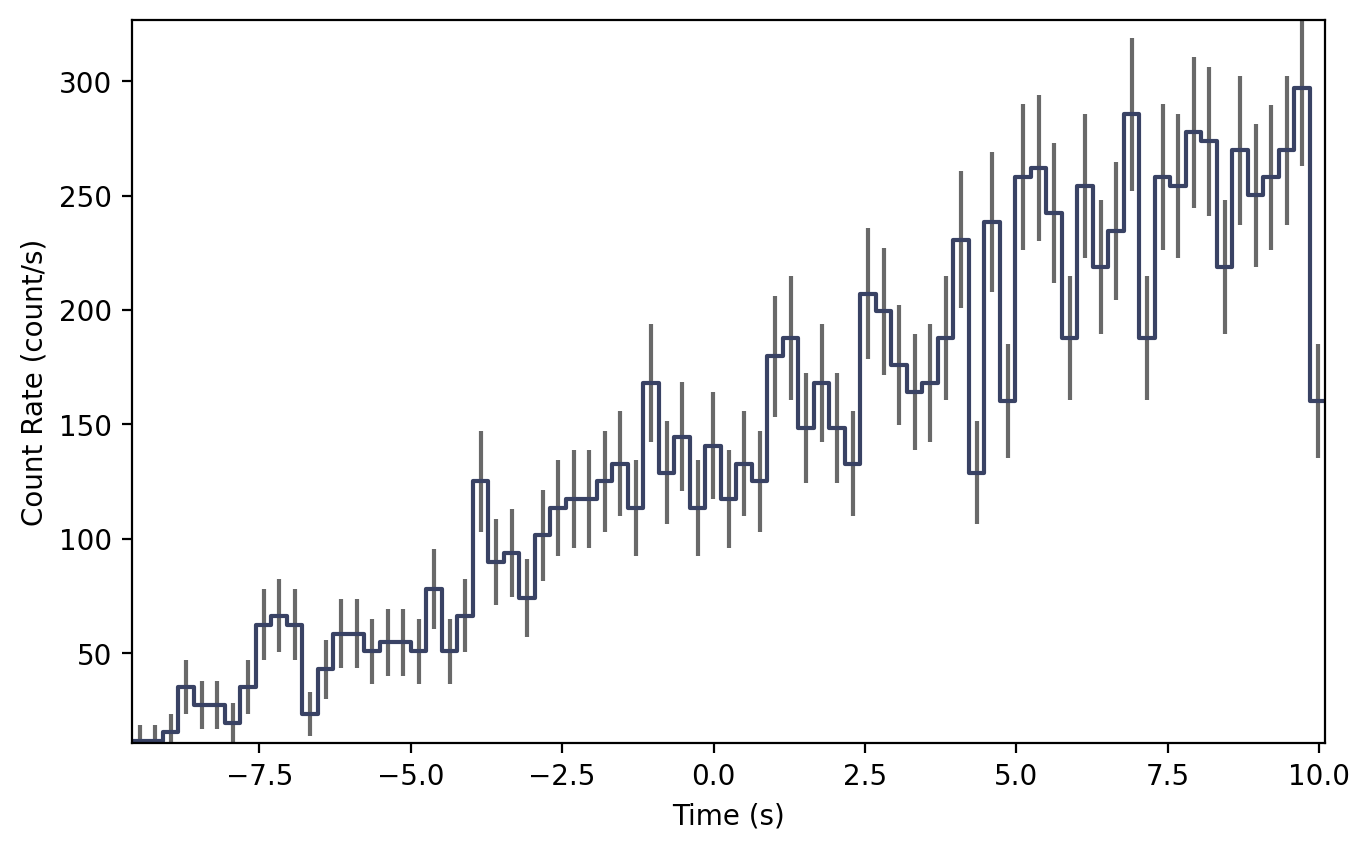
To illustrate what this looks like, we can bin the event data into a Phaii class and plot it. In this example, we will bin the data into 256 ms bins:

>>> from gdt.core.binning.unbinned import bin_by_time
>>> phaii = back_tte.to_phaii(bin_by_time, 0.256)

And now we can plot it as a lightcurve, integrated over all energies, with the Lightcurve plotting class:

>>> import matplotlib.pyplot as plt
>>> from gdt.core.plot.lightcurve import Lightcurve
>>> lcplot = Lightcurve(data=phaii.to_lightcurve())
>>> plt.show()

Simulating Source Event Data

To simulate source event data, we will use the TteSourceSimulator class. We must specify a detector response, spectral function and parameters, and temporal function and parameters. For the detector response, we will use the example detector response constructed in The Rsp Class, and then we will use a Band function (see Spectral Functions for more information on photon models). We will use the norris pulse model for the temporal function.

>>> from gdt.core.spectra.functions import Band
>>> from gdt.core.simulate.profiles import norris
>>> from gdt.core.simulate.tte import TteSourceSimulator
>>>
>>> # (amplitude, Epeak, alpha, beta)
>>> band_params = (0.01, 300.0, -1.0, -2.8)
>>> # (amplitude, tstart, trise, tdecay)
>>> norris_params = (0.05, 0.0, 0.1, 0.5)
>>> src_sim = TteSourceSimulator(rsp, Band(), band_params, norris, norris_params,
>>>                              deadtime=1e-6)

Now to simulate some data. To do so, we must specify a start and stop time (relative to time=0.0 s).

>>> src_events = src_sim.simulate(-10.0, 10.0)
>>> src_events
<EventList: 1245 events;
 time range (0.033597988692527656, 4.708158280056014);
 channel range (0, 3)>

Notice that even though we specified our simulation to span from T0-10 s to T0+10 s, that our data only starts at about T0 and ends about 5 s later. This is because we specified the start time to be at T0 (hence no source events prior to T0), and the Norris parameters lead to no events beyond T0+5 s.

As with the background we can also generate a higher-level PhotonList object:

>>> src_tte = src_sim.to_tte(-10.0, 10.0)
>>> src_tte
<PhotonList:
 time range (0.03792640604679924, 4.349491130015022);
 energy range (4.6, 2000.0)>

To illustrate what this looks like, we can bin the event data into a Phaii object and plot it. In this example, we will bin the data into 64 ms bins:

>>> from gdt.core.binning.unbinned import bin_by_time
>>> phaii = src_tte.to_phaii(bin_by_time, 0.064)

And now we can plot it as a lightcurve, integrated over all energies, with the Lightcurve plotting class:

>>> lcplot = Lightcurve(data=phaii.to_lightcurve())
>>> plt.show()

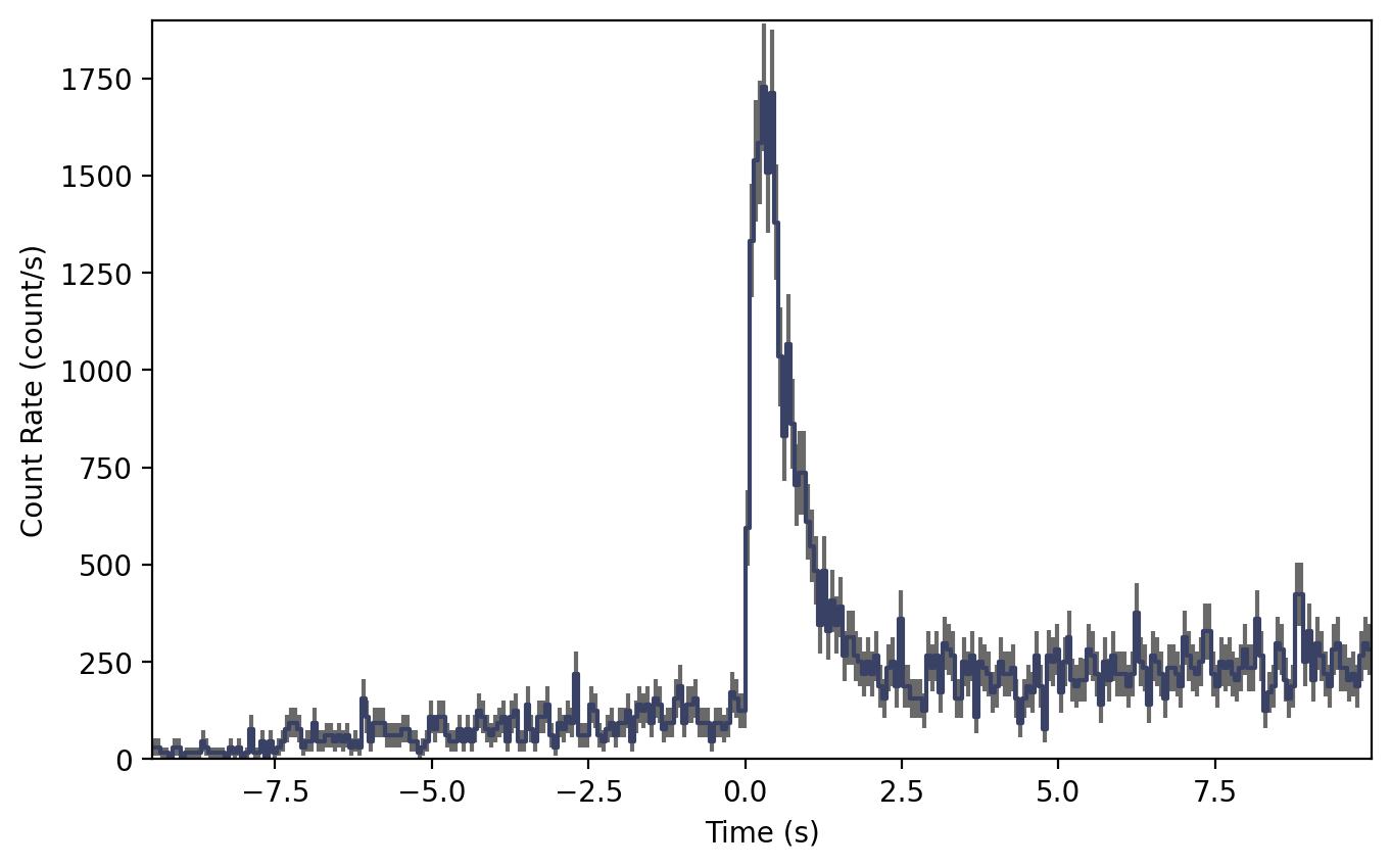
Simulating Background + Source Event Data

Usually we want to simulate the background and source combined. This is relatively easy to do once we have the our source and background simulators set up. All we need to do is merge the two simulated PhotonLists produced by the respective simulators:

>>> from gdt.core.tte import PhotonList
>>> back_tte = back_sim.to_tte(-10.0, 10.0)
>>> src_tte = src_sim.to_tte(-10.0, 10.0)
>>> total_tte = PhotonList.merge([back_tte, src_tte])

And finally, we can bin it into a Phaii object and plot:

>>> phaii = tte_total.to_phaii(bin_by_time, 0.064)
>>> lcplot = Lightcurve(data=phaii.to_lightcurve())
>>> plot.show()

Seeding Event Data

Users can set the random generator used to create each simulation with the rng keyword when initializing the TteSourceSimulator and TteBackgroundSimulator classes:

>>> import numpy as np
>>> rng = np.random.default_rng(seed=1)
>>> src_sim = TteSourceSimulator(rsp, Band(), band_params, norris, norris_params, deadtime=1e-6, rng=rng)
>>> back_sim = TteBackgroundSimulator(back_spec, 'Gaussian', linear, (1.0, 0.1), deadtime=1e-6, rng=rng)

This is useful in cases where reproducibility with a known seed is desired, such as for publicly shared simulation results.

Additionally, the random generator can be modified after initialization with the TteSourceSimulator.set_rng() and TteBackgroundSimulator.set_rng() functions:

>>> src_sim.set_rng(rng)
>>> back_sim.set_rng(rng)

In cases where the user does not provide their own generator, TteSourceSimulator and TteBackgroundSimulator will use np.random.default_rng() to create a default generator seeded by the computer’s clock time. This default generator will produce a different result whenever the simulation is performed at a different time. Simulations run at the same time will produce the same result, which can be problematic for users trying to run simulations as parallel processes. To avoid this, users should provide unique seeds to each simulation process when running in parallel. Below is an example of this for two parallel processes launched within a main function using Python’s multiprocessing module:

>>> import numpy as np
>>> import multiprocessing
>>>
>>> from gdt.core.data_primitives import ResponseMatrix
>>> from gdt.core.response import Rsp
>>> from gdt.core.background.primitives import BackgroundSpectrum
>>> from gdt.core.simulate.tte import TteBackgroundSimulator
>>> from gdt.core.simulate.profiles import linear
>>>
>>> def simulate(proc_id: int, n: int, rng: np.random.Generator, results: dict, sim: TteBackgroundSimulator):
>>>     sim.set_rng(rng)
>>>     results[proc_id] =  [sim.to_tte(-10, 10) for i in range(n)]
>>>
>>> if __name__ == "__main__":
>>>
>>>     rsp = ...
>>>     back_spec = ...
>>>
>>>     back_sim = TteBackgroundSimulator(back_spec, 'Gaussian', linear, (1.0, 0.1), deadtime=1e-6)
>>>
>>>     manager = multiprocessing.Manager()
>>>     results = manager.dict()
>>>
>>>     # perform 20 background simulations split across 2 parallel processes
>>>     rngs = np.random.default_rng().spawn(2)
>>>     procs = [multiprocessing.Process(target=simulate, args=(i, 10, rng, results, back_sim))
>>>              for i, rng in enumerate(rngs)]
>>>     [proc.start() for proc in procs]
>>>     [proc.join() for proc in procs]
>>>
>>>     for proc_id in sorted(results.keys()):
>>>         print(proc_id, results[proc_id])

Note that this requires the simulate() target method to be defined outside the main scope. Users looking for more flexibility or the ability to perform parallel processing within a Notebook should consider using the multiprocess dependency instead. This dependency is an extension of mulitprocessing that allows Manager() and Process() to be used in more scenarios, including within Notebooks.

Reference/API

gdt.core.simulate.tte Module

Classes

TteBackgroundSimulator(bkgd_spectrum, ...[, ...])	Simulate TTE or EventList data given a modeled background spectrum and time profile model.
TteSourceSimulator(rsp, spec_func, ...[, ...])	Simulate TTE or EventList data for a source spectrum given a detector response, spectral model and time profile model.

Class Inheritance Diagram