Fermi GBM PHAII Data (gdt.missions.fermi.gbm.phaii)

The primary science data produced by GBM can be summarized as a time history of spectra, which is provided temporally pre-binned (CTIME and CSPEC) or temporally unbinned (TTE). These data types are produced as “snippets” for every single trigger and are also provided continuously. CTIME and CSPEC are provided in daily chunks, and TTE are provided in hourly chunks (since late 2012). One of the most common things that a user of GBM data wants to do is look at this data (what we call a lightcurve) for one or more detectors over some energy range.

The CTIME and CSPEC data are temporally pre-binned data, which have 8 and 128 energy channels respectively. These data files can be read by the GbmPhaii class (or the aliased Ctime and Cspec classes).

>>> from gdt.core import data_path
>>> from gdt.missions.fermi.gbm.phaii import GbmPhaii
>>> # read a ctime file
>>> filepath = data_path.joinpath('fermi-gbm/glg_ctime_nb_bn120415958_v00.pha')
>>> ctime = GbmPhaii.open(filepath)
>>> ctime
<Ctime: glg_ctime_nb_bn120415958_v00.pha;
 trigger time: 356223561.133346;
 time range (-899.3424419760704, 1000.8578699827194);
 energy range (4.323754, 2000.0)>

Since GBM uses the FITS format, the data files have multiple data extensions, each with metadata information in a header. There is also a primary header that contains metadata relevant to the overall file. You can access this metadata information:

>>> ctime.headers.keys()
['PRIMARY', 'EBOUNDS', 'SPECTRUM', 'GTI']

>>> ctime.headers['PRIMARY']
CREATOR = 'GBM_SCI_Reader.pl v1.19' / Software and version creating file
FILETYPE= 'PHAII   '           / Name for this type of FITS file
FILE-VER= '1.0.0   '           / Version of the format for this filetype
TELESCOP= 'GLAST   '           / Name of mission/satellite
INSTRUME= 'GBM     '           / Specific instrument used for observation
DETNAM  = 'NAI_11  '           / Individual detector name
OBSERVER= 'Meegan  '           / GLAST Burst Monitor P.I.
ORIGIN  = 'GIOC    '           / Name of organization making file
DATE    = '2012-04-16T02:15:21' / file creation date (YYYY-MM-DDThh:mm:ss UT)
DATE-OBS= '2012-04-15 22:45:25.975' / Date of start of observation
DATE-END= '2012-04-15 23:17:06.175' / Date of end of observation
TIMESYS = 'TT      '           / Time system used in time keywords
TIMEUNIT= 's       '           / Time since MJDREF, used in TSTART and TSTOP
MJDREFI =                51910 / MJD of GLAST reference epoch, integer part
MJDREFF = '0.0007428703703703703' / MJD of GLAST reference epoch, fractional par
TSTART  =     356222661.790904 / [GLAST MET] Observation start time
TSTOP   =     356224561.991216 / [GLAST MET] Observation stop time
FILENAME= 'glg_ctime_nb_bn120415958_v00.pha' / Name of this file
DATATYPE= 'CTIME   '           / GBM datatype used for this file
TRIGTIME=     356223561.133346 / Trigger time relative to MJDREF, double precisi
OBJECT  = 'GRB120415958'       / Burst name in standard format, yymmddfff
RADECSYS= 'FK5     '           / Stellar reference frame
EQUINOX =               2000.0 / Equinox for RA and Dec
RA_OBJ  =                 30.0 / Calculated RA of burst
DEC_OBJ =                -15.0 / Calculated Dec of burst
ERR_RAD =                  3.0 / Calculated Location Error Radius

There is easy access for certain important properties of the data:

>>> # the good time intervals for the data
>>> ctime.gti
<Gti: 1 intervals; range (-899.3424419760704, 1000.8578699827194)>

>>> # the trigger time
>>> ctime.trigtime
356223561.133346

>>> # the time range
>>> ctime.time_range
(-899.3424419760704, 1000.8578699827194)

>>> # the energy range
>>> ctime.energy_range
(4.323754, 2000.0)

>>> # number of energy channels
>>> ctime.num_chans
8

We can retrieve the time history spectra data contained within the file, which is a TimeEnergyBins class (see 2D Binned Data for more details).

>>> ctime.data
<TimeEnergyBins: 14433 time bins;
 time range (-899.3424419760704, 1000.8578699827194);
 1 time segments;
 8 energy bins;
 energy range (4.323754, 2000.0);
 1 energy segments>

Through the Phaii base class, there are a lot of high level functions available to us, such as slicing the data in time or energy:

>>> time_sliced_ctime = ctime.slice_time((-10.0, 10.0))
>>> time_sliced_ctime
<Ctime:
 trigger time: 356223561.133346;
 time range (-10.240202009677887, 10.048128008842468);
 energy range (4.323754, 2000.0)>

>>> energy_sliced_ctime = ctime.slice_energy((50.0, 500.0))
>>> energy_sliced_ctime
<Ctime:
 trigger time: 356223561.133346;
 time range (-899.3424419760704, 1000.8578699827194);
 energy range (49.60019, 538.1436)>

As mentioned, this data is 2-dimensional, so what do we do if we want a lightcurve covering a particular energy range? We integrate (sum) over energy, and we can easily do this:

>>> lightcurve = ctime.to_lightcurve(energy_range=(50.0, 500.0))
>>> lightcurve
<TimeBins: 14433 bins;
 range (-899.3424419760704, 1000.8578699827194);
 1 contiguous segments>

Similarly, we can integrate over time to produce a count spectrum:

>>> spectrum = ctime.to_spectrum(time_range=(-10.0, 10.0))
>>> spectrum
<EnergyBins: 8 bins;
 range (4.323754, 2000.0);
 1 contiguous segments>

The resulting objects are TimeBins and EnergyBins, respectively, and see 1D Binned Data for more details on how to use them.

Of course, once we have produced a lightcurve or spectrum data object, often we want to plot it. For that, we use the Lightcurve and Spectrum plotting classes:

>>> import matplotlib.pyplot as plt
>>> from gdt.core.plot.lightcurve import Lightcurve
>>> lcplot = Lightcurve(data=lightcurve)
>>> plt.show()

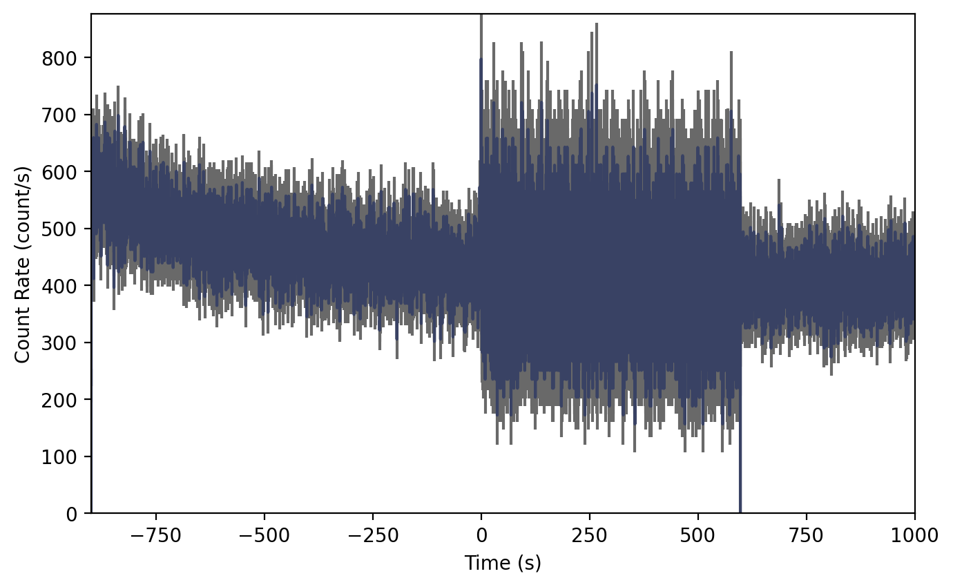
This plot may look odd without context. Since we are reading a trigger CTIME file, the file contains multiple time resolutions. Normally the CTIME data is accumulated in 256 ms duration bins, but starting at trigger time, the data switches to 64 ms duration bins for several hundred seconds, and then it goes back to 256 ms bins.

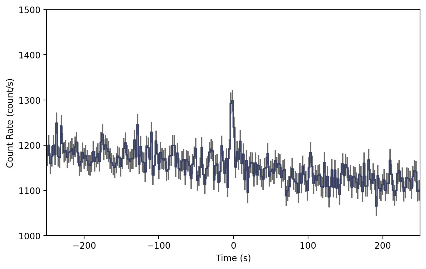
So maybe the native CTIME resolution is overkill because it’s hard to see the signal. We can make it easier to see the signal if we bin it up (see The Binning Package for details):

>>> from gdt.core.binning.binned import rebin_by_time
>>> # rebin the data to 2.048 s resolution
>>> rebinned_ctime = ctime.rebin_time(rebin_by_time, 2.048)
>>> lcplot = Lightcurve(data=rebinned_ctime.to_lightcurve())
>>> # zoom in
>>> lcplot.xlim = (-250.0, 250.0)
>>> lcplot.ylim = (1000.0, 1500.0)

After rebinning the data and zooming in a little, we can now easily see the GRB signal in the lightcurve.

Similarly, we can plot the count spectrum:

>>> from gdt.core.plot.spectrum import Spectrum
>>> specplot = Spectrum(data=spectrum)
>>> plt.show()

See Plotting Lightcurves and Plotting Count Spectra for more on how to modify these plots.

Finally, we can write out a new fully-qualified PHAII FITS file after some reduction tasks. For example, we can write out our time-sliced data object:

>>> time_sliced_ctime.write('./', filename='my_first_custom_ctime.pha')

For more details about working with PHAII data, see PHAII Files.

Reference/API

gdt.missions.fermi.gbm.phaii Module

Classes

GbmPhaii()	PHAII class for GBM time history spectra.
Ctime()	Class for GBM CTIME data.
Cspec()	Class for GBM CSPEC data.

Class Inheritance Diagram