Fermi GBM TTE Data (gdt.missions.fermi.gbm.tte)

TTE (Time-Tagged Event) data is basically a time-series of “counts” where each count is mapped to an energy channel. It is the temporally unbinned representation of CSPEC data (128 energy channels). We can read a TTE file with the GbmTte class, much the same way we can read Fermi GBM PHAII Data.

>>> from gdt.core import data_path
>>> from gdt.missions.fermi.gbm.tte import GbmTte
>>> filepath = data_path.joinpath('fermi-gbm/glg_tte_n9_bn090131090_v01.fit')
>>> tte = GbmTte.open(filepath)
>>> tte
<GbmTte: glg_tte_n9_bn090131090_v01.fit;
 trigger time: 255060563.149072;
 time range (-25.49109798669815, 300.73552399873734);
 energy range (4.3897294998168945, 2000.0)>

Since GBM uses the FITS format, the data files have multiple data extensions, each with metadata information in a header. There is also a primary header that contains metadata relevant to the overall file. You can access this metadata information:

>>> tte.headers.keys()
['PRIMARY', 'EBOUNDS', 'EVENTS', 'GTI']

There is easy access for certain important properties of the data:

>>> # the good time intervals for the data
>>> tte.gti
<Gti: 1 intervals; range (-25.49109798669815, 300.73552399873734)>

>>> # the trigger time
>>> tte.trigtime
255060563.149072

>>> # the time range
>>> tte.time_range
(-25.49109798669815, 300.73552399873734)

>>> # the energy range
>>> tte.energy_range
(4.3897294998168945, 2000.0)

>>> # number of energy channels
>>> tte.num_chans
128

We can retrieve the time-tagged events data contained within the file, which is an EventList class (see Event Data for more details).

>>> tte.data
<EventList: 422405 events;
 time range (-25.49109798669815, 300.73552399873734);
 channel range (0, 127)>

Through the PhotonList base class, there are a lot of high level functions available to us, such as slicing the data in time or energy:

>>> time_sliced_tte = tte.slice_time((-10.0, 10.0))
>>> time_sliced_tte
<GbmTte:
 trigger time: 255060563.149072;
 time range (-9.999035984277725, 9.998922020196915);
 energy range (4.3897294998168945, 2000.0)>

>>> energy_sliced_tte = tte.slice_energy((50.0, 300.0))
>>> energy_sliced_tte
<GbmTte:
 trigger time: 255060563.149072;
 time range (-25.48361200094223, 300.73552399873734);
 energy range (48.08032989501953, 304.6853332519531)>

Making a lightcurve using TTE data is slightly more complicated than it is for the pre-binned data because the TTE is temporally unbinned. So first the data has to be binned, and then it can be displayed. Here, we want to bin unbinned data, so we choose from the Binning Algorithms for Unbinned Data. For this example, let’s choose bin_by_time(), which simply bins the TTE to the prescribed time resolution. Then we can use our chosen binning algorithm to convert the TTE to a PHAII object

>>> from gdt.core.binning.unbinned import bin_by_time
>>> phaii = tte.to_phaii(bin_by_time, 1.024, time_ref=0.0)
>>> phaii
<GbmPhaii:
 trigger time: 255060563.149072;
 time range (-25.6, 301.056);
 energy range (4.3897294998168945, 2000.0)>

Here, we binned the data to 1.024 s resolution, and reference point at which to start the binning (in both directions) was at T0=0 s. Now that it is a GbmPhaii object, we can do all of the same operations that we could with CTIME or CSPEC data. For example, we can plot the lightcurve using the Lightcurve class:

>>> import matplotlib.pyplot as plt
>>> from gdt.core.plot.lightcurve import Lightcurve
>>> lcplot = Lightcurve(data=phaii.to_lightcurve())
>>> plt.show()

One thing to note, if we want to temporally rebin the data, we could certainly rebin the PHAII object, but in order to leverage the full power and flexibility of TTE, it would be good to (re)bin the TTE data instead to create a new PHAII object.

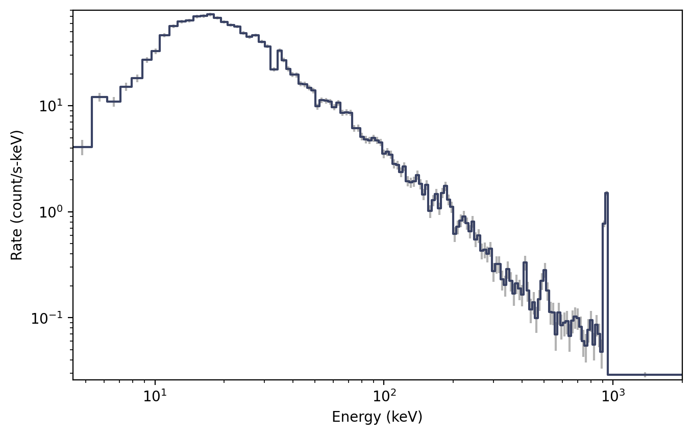
To plot the spectrum, we don’t have to worry about binning the data, since the TTE is already necessarily pre-binned in energy. So we can make a spectrum plot directly from the TTE object without any extra steps using the Spectrum class:

>>> from gdt.core.plot.spectrum import Spectrum
>>> # integrate over time from 0 - 10 s
>>> spectrum = tte.to_spectrum(time_range=(0.0, 10.0))
>>> specplot = Spectrum(data=spectrum)
>>> plt.show()

Perhaps the spectral resolution is a little bit higher than we need (i.e. if studying a weak source). We can rebin the count spectrum, but remember that the energy is pre-binned, so we need to use one of the Binning Algorithms for Binned Data. Here, we will use combine_by_factor(), which simply combines bins together by an integer factor:

>>> from gdt.core.binning.binned import combine_by_factor
>>> # rebin the count spectrum by a factor of 4
>>> rebinned_energy = tte.rebin_energy(combine_by_factor, 4)
>>> rebinned_spectrum = rebinned_energy.to_spectrum(time_range=(0.0, 10.0))
>>> specplot = Spectrum(data=rebinned_spectrum)
>>> plt.show()

See Plotting Lightcurves and Plotting Count Spectra for more on how to modify these plots.

Finally, we can write out a new fully-qualified GBM TTE FITS file after some reduction tasks. For example, we can write out our time-sliced data object:

>>> time_sliced_tte.write('./', filename='my_first_custom_tte.fit')

For more details about working with TTE data, see Photon List and Time-Tagged Event Files.

Reference/API

gdt.missions.fermi.gbm.tte Module

Classes

GbmTte()

Class for Time-Tagged Event data.

Class Inheritance Diagram